Bid Optimization In Broad Match Ad Auctions

ABSTRACT

Ad auctions in sponsored search support “broad match” that allows an advertiser to target a large number of queries while bidding only on a limited number. While giving more expressiveness to advertisers, this feature makes it challenging to optimize bids to maximize their returns: choosing to bid on a query as a broad match because it provides high profit results in one bidding for related queries which may yield low or even negative profits.

We abstract and study the complexity of the bid optimization problem which is to determine an advertiser’s bids on a subset of keywords (possibly using broad match) so that her profit is maximized. In the query language model when the advertiser is allowed to bid on all queries as broad match, we present an linear programming (LP)-based polynomialtime algorithm that gets the optimal profit. In the model in which an advertiser can only bid on keywords, ie., a subset of keywords as an exact or broad match, we show that this problem is not approximable within any reasonable approximation factor unless P=NP. To deal with this hardness result, we present a constant-factor approximation when the optimal profit significantly exceeds the cost. This algorithm is based on rounding a natural LP formulation of the problem. Finally, we study a budgeted variant of the problem, and show that in the query language model, one can find two budget constrained ad campaigns in polynomial time that implement the optimal bidding strategy. Our results are the first to address bid optimization under the broad match feature which is common in ad auctions.

Categories and Subject Descriptors

General Terms

Algorithm, Theory, Economics

Keywords

Sponsored Search, Ad Auctions, Optimal bidding, Bid Optimization

1. INTRODUCTION

Sponsored search is a large and thriving market with three distinct players. Users go to search engines such as Yahoo! or Google and pose queries; in the process, they express their intention and preferences. Advertisers seek to place advertisements and target them to users’ intentions as expressed by their queries. Finally, search engines provide a suitable mechanism for doing this. Currently, the mechanism relies on having advertisers bid on the search issued by the user, and the search engine to run an auction at the time the user poses the query to determine the advertisements that will be shown to the user. As is standard, the advertiser only pays if the user clicks on their ad (the “payper-click” model), and the amount they pay is determined by the auction mechanism, but will be no larger than their bid.

In this paper, we assume the perspective of the advertiser. The advertisers need to target their ad campaigns to users’ queries. Thus, they need to determine the set S of queries of their interest. Once that is determined, they need to strategize in the auction that takes place for each of the queries in S. A lot of research has focused on the game theory and optimization behind these auctions, both from the search engine [2, 20, 7, 1, 13, 5] and advertiser [4, 9, 6, 14] points of view. There has been relatively little prior research on how advertisers target their campaign, i.e., how they determine the set S.

The criterion for choosing S is for the advertiser to pick a set of keyphrases that searchers may use in their query when looking for their products. The central challenge then is to match the advertisers keyphrases with the potential queries issued by the users. It is difficult if not impossible for the advertisers to identify all possible variations of keyphrases that a user looking for their product may use in their query. As an example, consider a vendor who chooses the keyphrase tennis shoes. Users searching for them may use singular or plural, synonyms and other variations (“clay court footwear”), may misspell (“tenis shoe”), use extensions (“white tennis shoes”) or reorder the words (“shoes lawn tennis”). In fact, users may even search using words not found in the keyphrase (“Wimbledon gear”, “US Open Shoes”, “hard court soles”), and may still be of interest to the advertiser. These artifacts such as plurals, synonyms, misspellings, extensions, and reorderings are very common,

and the problems get compounded since typical ad campaigns comprise several keyphrases, each with its own set of artifacts.

Major search engines help advertisers address this challenge by providing a structured bidding language. While the specific details differ from search engine to search engine [21, 22, 23], at the highest level, the bidding language supports two match types: exact and broad. In exact matchtype (called “exact” in MSN AdCenter and Google, and “standard” in Yahoo), ad would be eligible to appear when a user searches for the specific keyphrase without any other terms in the query, and words in the keyphrase need to appear in that order. In broad matchtype (called “broad” in MSN, related to “phrase” and “broad” in Google, and “advanced match type” in Yahoo), the system automatically makes advertisers eligible on relevant variations of their keyphrases including for the various artifacts listed earlier, even if the search terms are not in the keyphrase lists. Thus, the search engines automate the aspect of detecting artifacts and matching the query to keyphrases of interest to advertisers.1 Thus the task of advertisers becomes determining the keyphrases and choosing the match type on each.

The question we address here is, how does an advertiser bid in presence of these match types? Say each query q has a value v(q) per click for the advertiser that is known to the advertiser and is private. Further, we let c(q) be the expected price per click and let n(q) be the expected number of clicks. These are statistical estimates provided by the search engines [24, 25, 26]. Then, we consider two optimization problems: (i) in one variant, we assume that the advertiser wishes to maximize their expected profit, that is, P q (v(q) − c(q))n(q), and (ii) in the other variant, given a budget B for the advertiser, we assume that the advertiser wishes to maximize their expected value, that is, P q v(q)n(q) subject to the condition that the expected spend P q c(q)n(q) does not exceed the budget.

The technical challenge arises due to query dependencies. When one bids on a keyphrase for query q, as a result of a broad match, it may apply to query q ′ as well. The advertiser has different values v(q) and v(q ′ ) on these because users for q and q ′ differ on their intentions and therefore on their respective values to the advertiser. So, the advertiser may make good profit on q and may wish to bid on that query, but is then forced to implicitly bid on q ′ as well, and may even make negative profit on q ′ ! Under what circumstances is it now desirable for the advertiser to bid for q?

Note that query dependence is a fundamental aspect of sponsored search since advertisers can realistically only choose and strategize on a small set of keyphrases because of the effort involved, and have to typically rely on the search engine to carefully apply their strategy to variants of their keyphrases. But beyond that, even an ad campaign that is willing to exert a lot of effort and use a large number of keyphrases or relies on a search engine to provide rich bidding languages [11] will still find it impossible to include all search variations of the keyphrases as exact matches, and must necessarily rely on broad match for the variations that

search users develop and prefer over time. Thus, the advertisers bid implicitly on queries on which they can not directly control the tradeoff between the cost and the value.

Query dependence introduces a complex optimization problem of trading off the benefits of bidding on a keyphrase against the impact of bidding on its dependent queries. In the sponsored search world, there is a keen awareness of this complexity of bidding, and most search engines and thirdparty bidding agents provide detailed tips and guidelines for advertisers [27, 28]. Beyond these guidelines, what is missing is a clear theoretical understanding of the tradeoffs and the complexity of the bidding problem that advertisers face.

We initiate principled study of bidding in presence of broad matches. Specifically, our contributions are as follows.

1. We abstract two models — query and keyword language models — to study bidding optimization problems.

In the query language model, the advertiser bids directly on user queries and wishes to determine which query if any to bid on, to maximize expected profit. This models both the theoretical extreme where an advertiser can bid on any of the queries the search engine will see, and the practical reality where the advertiser has a select set of queries in mind and wishes only to optimize within that set. In the keyword language model, advertisers may bid only on a subset of queries, and broad match implicitly derives bids as needed. This directly models the common reality.

2. We present efficient, polynomial time algorithms for the bid optimization problem under these two models.

In query bidding, we get a polynomial-time algorithm that maximizes the profit, using a reduction to the well-known Min-Cut problem in graphs. This is in contrast to the poor performance of natural greedy algorithms for this problem. We also study the budgeted variant of the problem, and propose a novel strategy using two distinct budgeted ad campaign that gets the optimal profit. We do so by studying the structure of the basic feasible solutions of a corresponding linear programming formulation of the problem.

For keyword bidding, we show that even limited instances are NP-Hard to not only optimize, but even to approximate; to deal with this hardness result, we present a constant-factor approximation when advertisers profit following an optimal bid is considerably greater than her cost. This result is based on applying a randomized rounding method on the optimal fractional solutions of the linear programming relaxation of the problem.

These represent the first known theoretical results for the problem of bid optimization in presence of broad matches, a problem advertisers face now since this feature is offered by the major search engines. Prior research in bid optimization for advertisers [4, 6, 16] primarily focused on determining suitable bids for exact match types and does not study the query dependence and implicit bids; [9, 14] studied the problem of maximizing the number of clicks, and not the profit which is the more standard metric. At the technical core, our challenge is to tradeoff positive profit from

¹These match types may be further modified by ensuring that the ad be not shown on occurrence of certain keywords in the query; this feature (called “negative” in MSN and Google or “excluded” by Yahoo) and other targeting criteria associated with keyphrase campaigns do not change the discussion and the results here.

bidding on a keyphrase that applies to one query q against possibly a negative profit from the implied bids of broad match on queries q’. This query dependence is a novel feature in sponsored search auctions, not explicitly studied in prior literature, and our results for this problem may have applications beyond, in the general auction theory area.

Finally, we report experimental results on a small family of instances of the bid optimizations problem, and compute the optimal bidding using the integer linear programming formulation. Our main observation in these experiments is that by considering only the broad match, we do not lose much in the maximum profit of the solution. This supports our hope that under reasonable circumstances (similar to the ones in our experiments), considering only broad match is effective, and in turn, that would enable advertisers to focus on campaigns with small lists of keyphrases.

2. MODEL

We consider the optimization problems that an advertiser faces while bidding in an auction for queries with a broad match feature.

The Advertiser. We consider a single advertiser who is interested in showing her ad to users after they search for queries from a set Q. The advertiser has some utility from having a user click on her ad. In reality, clicks associated with different queries may bring have utility to the advertiser; The advertiser has a value of v(q) units of monetary value associated with a ‘click’ that follows a query $q \in Q$ .

We assume a posted price model where prices are posted and the search volume of every query as well as its click through rate (i.e., the probability that users would click her ad) are known to the advertiser. Namely, every query q is associated with a pair of parameters, known to the advertiser, (c(q), n(q)), where c(q) is the per click cost of q, and n(q) is the expected number of clicks that would result from winning q (the expected number of clicks can be determined from the search volume of q and the advertiser’s specific click through rate for q).

Thus, when an advertiser wins a query q, her overall profit ² from winning, denoted w(q) is

$w(q) = (v(q) - c(q)) n(q) .$

Note that although each query has a positive value, winning it may result an overall negative profit.

Bidding languages. A bidding language is a way for an advertiser to specify her value or willingness to pay for queries. Eventually, the auctioneer needs to have a bid for every possible query ³. The choice of a bidding language is critical for the auction mechanism. At the one extreme, it may be infeasible to allow an advertiser to specify explicitly her value for every possible query. On the other hand, a language that is too restrictive would not allow an advertiser to communicate her preferences properly.

In order to study the complexity of the optimal bidding in the broad match framework while taking into account the intersections among broad matches for different keywords, we first consider a bidding language in which an advertiser can specify a bid for every query q but only as a broadmatch. We refer to this language as the $query\ language$ .

To allow the most accurate description of an advertisers value per query, the ultimate way is to let the advertiser specify all possible queries with exact or broad match, and a monetary bid for each of them. If an advertiser is allowed to bid on each type of query as an exact match as well as broad match, she can decide for each query independent of the other queries, and the complexity of the bidding problem is not captured in such bidding language.

To capture the complexity of the optimal bidding problem and the fact that advertisers may only bid on a subset of queries, we study the keyword language that allows advertisers to place a bid only on (single) keywords or short phrases. More precisely, in the keyword language, we assume that advertisers are allowed to bid only on a subset $S \subset Q$ of queries.

A further improvement of this language would allow the advertiser to specify, besides a value bid for $s \in S$ , whether s is to be matched exactly or broadly.

A bid $b \in \mathbb{R}_+^{|Q|}$ in some bidding language is associated with a set of ‘winning queries’ denoted by $\varphi(b) = \{q \in Q \mid b(q) \ge c(q)\}$ . A subset T of queries which is a winning set of some bid b is referred to as a feasible winning set. The utility associated with a winning set T is

$u(T) = \sum_{q \in T} (v(q) - c(q)) n(q),$

where $v(\cdot)$ and $n(\cdot)$ are advertiser specific.

A feasible winning set with optimal utility is referred to as an optimal winning set.

The Auction. For every query, the auctioneer should decide the bid of every advertiser. This decision is easy for queries on which the advertiser bids explicitly (as an exact match). However, for the queries that the advertiser has not bid directly, but only through a broad match framework, the auctioneer should compute an appropriate bid for the advertiser to participate in the auction.

A natural way for setting such a value is to aggregate the bid values of all the phrases matched by the query. While there are several choices for the aggregation method, in this paper, we consider the max aggregation operator — when a query q matches phrases $w_1, \ldots, w_k$ from the advertiser list of phrases, its bid is interpreted as $b(q) = \max_i b(w_i)$ .

We can now state formally the bid optimization problem. Given advertiser’s specific data (A set Q, value for queries v, search volume and click through rates $n(\cdot)$ ) and a bidding language $\mathcal{L}$ , an optimal bid $b^*$ , is a feasible bid in the language $\mathcal{L}$ that maximizes the advertisers’ utility from winning a set $\varphi(b)$ of queries. Formally,

b^* \in argmax_{b \in \mathcal{L}} \{ u(\varphi(b)) \}. \tag{2.1}

Query dependencies. We say that a query q depends on a query q’ if winning query q’ implies winning query q. In the broad match auction in which the bid interpretation strategy is done using the max operator, this happens if q matches q’ broadly, and its cost c(q) is less than that of c(q’). In other words, if a bid b wins q’, it must be that $b(q') \geq c(q')$ , but

$^{^{2}\}mathrm{In}$ this paper, we use terms utility and profit interchangably.

$^{^{3}}$ A bid of 0 for a query may be regarded as the default in a case where the advertiser is not explicitly interested in a query q and nor in queries that q match broadly.

the interpreted bid for q is then at least $b(q') \geq c(q)$ since $c(q') \geq c(q)$ , hence the bid b must be winning q as well. As a result, the cost structure incurs a set of pairs (q’,q) where the first entry of each pair $q' \in S$ is a valid phrase in the bidding language and the second entry is a valid query in the set of queries Q such that winning query q’ implies winning query q. This set of pairs is denoted by C and formally:

$\mathcal{C} = \{(q',q)|q' \in S, q \in Q, q \text{ matches } q' \text{ broadly }, c(q') \geq c(q)\}.$ Moreover, we define $D(q) = \{q'|(q',q) \in \mathcal{C}\}$ , and $N(q) = \{q'|(q,q') \in \mathcal{C}\}.$

Budget-constrained Ad Campaigns. A variant of the optimal bidding problem in the broad match framework is to find a set of queries to bid on that maximizes the total value of the gueries won by the advertiser subject to a budget constraint, i.e, our goal is to bid on a subset T of queries to maximize $\sum_{q \in T} v(q)n(q)$ subject to the budget constraint $\sum_{q \in T} c(q) n(q) \leq B$ . To handle such a budget constraint, we assume that one can run a budget-constrained ad campaign by bidding on a subset T of keywords and setting a budget B. Assuming $B' = \sum_{q \in T} c(q)n(q)$ , there are two possibilities in this budget-constrained ad campaign: (i) If $B' \leq B$ , the auction is run in a normal way and the value from this ad campaign for the advertiser is $\sum_{q \in T} v(q) n(q)$ , (ii) On the other hand, if B’ > B, we assume that the queries arrive at the same rate and as a result, for each query, we get $\frac{B'}{B}$ fraction of the value of an ad campaign without the budget constraint. In other words, the value that the advertiser gets is $\sum_{q\in T}v(q)n(q)\frac{B'}{B}$ . We can also interpret the above assumption by a throttling method in which, in order to cope with the budget constraint, at each step, we let the advertiser participate in the auction with probability $\frac{B'}{R}$ .

3. BIDDING IN THE QUERY LANGUAGE

In this section, we study the query language that allows placing a bid on every query. We observe that in the query language, the task of computing an optimal bid is equivalent to that of computing an optimal winning set: Given an optimal feasible set T set a bid b(q)=c(q) for every query $q\in T$ with positive weight and b(q)=0 otherwise.

Lemma 3.1. A bid b derived from an optimal winning set T, as described above, is an optimal bid.

PROOF. By construction, the bid b wins all the queries with positive weight from T, and every other query must belong to T (otherwise T would not be feasible). $\square$

We therefore consider algorithms for computing an optimal feasible winning set. First, we consider a greedy algorithm, denoted by Max-Margin Greedy. Initially, Max-Margin Greedy sets the winning set to be empty. Then, iteratively, it adds a bid on a query with the highest marginal benefit to the winning set utility. Unfortunately, Max-Margin Greedy fails to compute an optimal winning set due to the following example.

Example. Consider a set Q of queries which contains n keywords and another $\binom{n}{2}$ queries, each of which is a pair of keywords. The cost of each query is set to $1. Hence, the query dependencies is such that winning a keyword implies

winning the set of n-1 queries made of pairs of keywords in which this keyword appears. The value of a keyword is set to $2; The value of a each pair is set to 1-1.5/n. So, every keyword attains a positive utility of $1, and every pair causes a loss of $1.5/n. Initially, Max-Margin Greedy’s bid is empty. At this point Max-Margin Greedy is stuck—every single query it adds to the winning set results in a negative overall utility. Thus, this instance, Max-Margin Greedy would yield 0 utility. An optimal solution wins all the queries and has a utility of $n \times (2-1) - \binom{n}{2} (1 - \frac{1.5}{n} - 1) = \frac{n-3}{4}$ .

One can explore other variants of greedy algorithms for this problem. For example, a natural greedy algorithm is Max-Rate Greedy algorithm: Initially set the winning set to the empty set, and then iteratively, add a bid on a query with the highest ratio of marginal profit over the marginal cost, or the query with the highest ratio of marginal value over marginal cost. We note that all these iterative greedy algorithms pefrom poorly for the above example. Even a significant look-ahead will not resolve this bad example.

We turn to the next algorithm OptBid1 for computing an optimal winning set. OptBid1 is a solution to the following integer linear program:

ILP : $\max \sum_{q_i \in Q} X_{q_i} w(q_i)$ For every pair $(q_j, q_i) \in \mathcal{C}$ : $X_{q_i} - X_{q_j} \ge 0$
$\forall q_i \in Q : X_{q_i} \in \{0, 1\}$ (3.1)

For every query q, an integral variable $X_q$ is a 0-1 variable which is equal to 1 if and only if q belongs to the winning set of queries. In order to solve the above ILP, we relax it to a linear program where instead of integer 0-1 variables, we have fractional $X_q$ variables with values between 0 and 1 $(0 \le X_q \le 1)$ . Here, we observe that the integrality gap of this linear programming relaxation is 1, i.e., for any instance of this linear program, there exists an optimal solution $X^*$ in which all the values are integer $X_q^* \in \{0,1\}$ for all $q \in Q$ .

Lemma 3.2. The integrality gap of the linear programming relaxation of the ILP 3.1 is one.

PROOF. The lemma follows from the fact the the constraint matrix of the LP relaxation of ILP 3.1 is totally unimodular⁴. A sufficient condition for a matrix to be totally uni-modular is that every row has either two non-zero entries, one is 1 and the other -1, or a single non zero entry with value 1 or -1. An integer program whose constraint matrix is totally uni-modular and whose right hand side is integer can be solved by linear programming since all its basic feasible solutions are integer (see [15] pp. 316). $\square$

The above lemma implies the following polynomial-time algorithm OptBid1 for optimal bidding in the query language: compute a basic feasible solution $X^*$ of the LP relaxation of ILP 3.1, and find a bidding strategy corresponding to the winning set of $X^*$ , i.e., $\{q \in Q | X_q^* = 1\}$ .

The running time of Algorithm OptBid1 is that of solving a linear program with $\Omega(|Q|^2)$ constraints, which although polynomial in |Q|, might be inefficient. Next, we present a faster algorithm, OptBid2.

$^{^4}$ A matrix A is totally uni-modular if every square submatrix of it is uni-modular, i.e., every submatrix has a determinant of 0, -1 or +1.

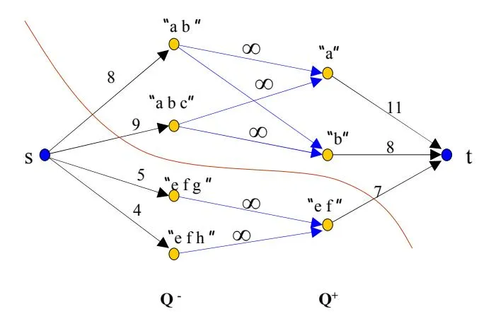
Figure 1: An example of running algorithm Opt-Bid2 on the set of queries (with the following profit: $\{(a, 11), (b, 8), (ab, -8), (abc, -9), (ef, 7), (efg, -5), (efh, -4)\}\}$ and dependency graph as illustrated. ObtBid2 will choose the winning set $\{a, b, ab, abc\}$ . The optimal bid is $\{(a, 11), (b, 8)\}$ .

For the purpose of presenting Algorithm OptBid2, we define a weighted flow graph G = (V, E), derived from the input. The vertex set of G is $V = \{s, t\} \cup Q^+ \cup Q^-$ , where s is a source node, t is a target node and $Q^+$ and $Q^-$ are the sets of queries with positive/non-positive weights respectively, i.e., $Q^+ \equiv \{q \mid w(q) > 0\}$ . The source vertex s is connected to each vertex $q \in Q^-$ with an edge of weight |w(q)| = |(v(q) - c(q))n(q)|. The target vertex t is connected with each vertex $p \in Q^+$ with an edge of weight w(p). Two vertices $q \in Q^-, p \in Q^+$ are connected with an edge of weight $\infty$ if and only if $(p,q) \in \mathcal{C}$ .

Algorithm OptBid2

• 1. Compute a min-cut of G. Let S, T be the two sides of the cut.
• 2. Assume, without loss of generality, that $t \in T$ . Return $T \setminus \{t\}$ , that is, the set of queries that are on the same side of the cut as t is an optimal winning set.

The running time of Algorithm OptBid2 is that of mincut, i.e., $O(|Q|^3)$ [18].

THEOREM 3.3. Algorithm OptBid2 finds an optimal winning set.

PROOF. We show T is an optimal winning set using the dual program of ILP.

DUAL : $\min \sum_{q \in Q^+} Z_q$

DUAL : $\min \sum_{q \in Q^+} Z_q$

$\forall q \in Q^+$ : $\sum_{q':(q,q') \in \mathcal{C}} Y_{q,q'} + Z_q \ge w(q)$

$\forall q' \in Q^- : \sum_{q:(q,q') \in \mathcal{C}} Y_{q,q'} \le -w_{q'} \text{ (Notice that } w_{q'} \le 0)$

$\forall (q, q') \in \mathcal{C} : Y_{q,q'} \ge 0$ $\forall q \in Q^+ : Z_q \ge 0$

Let $f = (f_e)_{e \in E}$ be a maximum flow in G, with value c. For every $(q,q') \in \mathcal{C}$ , set $Y_{q,q'} := f_{q,q'}$ and for every $q \in Q^+$ , set $Z_q := w(q) - \sum_{q' \mid (q,q') \in \mathcal{C}} Y_{q,q'}$ . It is straightforward to verify that this is a feasible solution of DUAL with value

$\sum_{q \in Q^+} w(q) - c.$ Now, observe that T is a feasible set in the query language. For every pair $(q, q') \in \mathcal{C}$ , we have that if $q \in T$ then also $q' \in T$ . Otherwise, the edge (q, q’), with weight $\infty$ , would be part of the cut. Thus, the value of the min cut is

$c = \sum_{q \in Q^- \cap T} |w(q)| + \sum_{q \in Q^+ \backslash T} w(q).$

and therefore.

$u(T) = \sum_{q \in T} w(q) = \sum_{q \in Q^+} w_q - \sum_{q \in Q^+ \setminus T} w(q) + \sum_{q \in Q^- \cap T} w(q)$ $= \sum_{q \in Q^+} w_q - c.$

We already found a feasible solution for the dual of ILP, with the same value. We therefore conclude, using the weak duality theorem, that T is an optimal solution of ILP. $\square$

BIDDING IN THE KEYWORD LANGUAGE

In this section, we study optimal bidding for the keyword language, where the advertiser is restricted to bid on a subset of (possibly short) queries $S \subset Q$ .

Note that in the case that all queries have positive utility, the optimal bid is trivial by simply placing a high bid for every query in S. In addition, finding the optimal bid when all queries are associated with a negative utility is trivial (a bid of $0 for every phrase in S is optimal). Moreover, in the case of uniform value from every query, the optimal bid is easy — a uniform bid equal to the uniform value guarantees winning every query with positive weight and losing every query with negative weight, which is of course optimal. In realistic settings, some queries have positive utility and some have negative utility. In this case the problem of finding the optimal bid becomes intractable. More precisely, as we show now, even when the set of queries Q is made up from single keywords and pairs of keywords, this problem becomes hard to approximate within a factor of $|S|^{1-\epsilon}$ , for every $\epsilon > 0$ :

Theorem 4.1. In the keyword language broad match framework, it is NP-hard to approximate the optimal value of the optimal bidding problem within a factor of $|S|^{1-\epsilon}$ , for any $\epsilon > 0$ .

PROOF. We give a factor-preserving reduction to the independent set problem. Given a graph G with n nodes, and m edges, we construct the following instance of our problem: put a singleton keyword for each node v of G with weight $w_v = -(deg(v) - 1)$ , and put a query consisting of a pair of keywords corresponding to each edge e of G with weight 1. The maximum value we can get from picking a keyword is 1, and we get this value if all of its neighbors do not appear in the output. It can be seen that the optimum solution is an independent set of nodes (since otherwise, we get zero or negative from a picked node), and as a result, the maximum value is the same as the size of the independent set. $\square$

4.1 A Constant-Factor Approximation

In this section, in light of the above hardness result, we design a constant-factor approximation algorithm for a special case of the optimal bidding problem in the keyword language in which the cost part of the optimal solution is less than $\frac{1}{c}$ of the value part of the optimal solution, for some constant c > 1. Recall that $D(q) = \{q'|q' \in S, (q',q) \in \mathcal{C}\}$ . Our algorithm is constant-factor approximation if for any query $q \in Q \setminus S$ , |D(q)| is less than a constant c’. We present our result for the case that each query $q \in Q$ can be in the broad-match set of at most two queries $q_1, q_2 \in S$ , i.e., $|D(q)| \leq 2$ . However, our result can be extended to more general settings in which query $q \in Q$ can be the broad match for a constant number of queries $q_1, \ldots, q_{c'} \in S$ (for a constant c’).

Based on the above discussion, we assume that $|D(q)| \le 2$ for any query $q \in Q$ . Note that the hardness result of the keyword language holds even for instances in which $|D(q)| \le 2$ for all queries $q \in Q$ . Also, let $E = \{c(q)|q \in Q\}$ . Our algorithm is based on a linear programming relaxation of the optimal bidding problem for the keyword language. The integer linear program is as follows:

ILP-Approx max $\sum_{s \in S} (Z_s^{c(s)} + R_s) w_s$ $+ \sum_{q \in Q \setminus S} Y_q w_q$ $\forall q \in Q \setminus S, (s, q) \in \mathcal{C}, (r, q) \in \mathcal{C} \qquad Y_q \leq Z_s^{c(q)} + Z_r^{c(q)}$ $\forall q \in Q \setminus S, (s, q) \in \mathcal{C} \qquad Y_q \geq Z_s^{c(q)}$ $\forall s \in S, p, p' \in E \qquad Z_s^p = \sum_{t \in E, t \leq p} W_s^t$ $\forall s \in S, p \in E \qquad Z_s^p + R_s \leq 1$ $\forall q \in Q \setminus S \qquad Y_q \in \{0, 1\}$ $\forall s \in S, p \in E \qquad W_s^p, Z_s^p \in \{0, 1\}$ $\forall s \in S, p \in E \qquad W_s^p, Z_s^p \in \{0, 1\}$ $(4.1)$

Where the variables correspond to the following:

• $W_s^p$ for any $s \in S$ is the indicator variable corresponding to the bid of p on query s (as a broad match),
• $Z_s^p$ for any $s \in S$ is the indicator variable corresponding to the bid of at most p on query s (as a broad match),
• $R_s$ for any $s \in S$ is the indicator variable corresponding to the exact match bid on query s,
• $Y_q$ for any $q \in Q \setminus S$ is the indicator variable corresponding to winning query q (as a result of bidding on queries in S).

We relax the integer 0-1 variables in this integer linear program to fractional variables between zero and one, and then compute an optimal fractional solution for this LP relaxation. Then we round this fractional solution to construct a feasible (integral) bidding strategy.

Rounding to an Integral Solution. Given a fractional solution (V, Z, W, Y) to the LP, we round it to an integral solution (V’, W’, Z’, Y’) as follows: for every query $s \in S$ , we set $V'_s = 1$ with probability 1, and $V'_s = 0$ otherwise. If $V'_s = 1$ , we set $W'^p_s = 0$ for all $p \in E$ . Otherwise, for each $s \in S$ , for all $p^* \in E$ , we choose $p^*$ with probability proportional to $W^{p^*}_s(1-\epsilon)$ (for an appropriate small constant $\epsilon$ that will be determined later) and set $W'^{p^*}_s = 1$ , and for any $p \neq p^*$ , we set $W'^p_s = 0$ . After setting all W’ variables, for each $p \in E$ and $s \in S$ , we set $Z'^p_s = \sum_{t \in E, t \leq p} W'^t_s$ . Finally, for any $q \in Q \setminus S$ , $Y'_q = 1$ if and only if $Z'^{c(q)}_s = 1$ for some

$s \in S$ , such that $s \in D(p)$ (or equivalently $(s,q) \in \mathcal{C}$ ). It is not hard to see that the above rounded integral solution correspond to a feasible bidding strategy. In particular, we can implement this bidding strategy by putting an exact match bid of b(s) = c(s) for any $s \in S$ if $R'_s = 1$ (i.e., with probability $R_s$ ) and then by putting a broad match bid of b(s) = p for query $s \in S$ if $W'^p_s = 1$ (i.e., with probability $W^p_s(1-\epsilon)$ ).

A query $s \in S$ is selected if bid b(s) for this query is at least c(s). As a result, a query $s \in S$ is selected with probability $(1-\epsilon)Z_s^{c(s)} + R_s$ . Moreover, for a query $q \in Q \setminus S$ for which $(s,q) \in \mathcal{C}$ and $(r,q) \in \mathcal{C}$ , query q is selected if the bid for either of the queries s or r is at least c(q), i.e., with probability

$\Pr[\ query\ q\ is\ selected\ ] = 1 - (1 - (1 - \epsilon)Z_s^{c(q)})(1 - (1 - \epsilon)Z_r^{c(q)}) = (1 - \epsilon)(Z_s^{c(q)} + Z_r^{c(q)}) - (1 - \epsilon)^2 Z_r^{c(q)} Z_s^{c(q)}.$

Therefore, the expected utility of the solution after implementing the integral solution (V’, W’, Z’, Y’) (or bidding as desribed above) is:

$\sum_{s \in S} ((1 - \epsilon)Z^{c(s)} + R_s) w_s + \sum_{q \in Q \setminus S; r, s \in D(q)} \left( (1 - \epsilon)(Z_s^{c(q)} + Z_r^{c(q)}) - (1 - \epsilon)^2 Z_s^{c(q)} Z_r^{c(q)} \right) w_q$

Next, we derive a lower bound and an upper bound on the probability that the bid generated as above, wins query q. We will show that

$Y_q(1-\epsilon)(1-\frac{1}{2}(1-\epsilon)) \le \Pr[q \text{ is selected }] \le (1-\epsilon)2Y_q.$

$(4.2)$

Consider the following set of inequalities that hold for every query q that depends on queries $s, r \in D(q)$ :

$Z_s^{c(q)} Z_r^{c(q)} \le \sqrt{Z_s^{c(q)} Z_r^{c(q)}} \le$

$\frac{Z_s^{c(q)} + Z_r^{c(q)}}{2} \le Y_q \le Z_s^{c(q)} + Z_r^{c(q)},$ (4.3)

The first inequality follows the constraints $0 \le Z_s^{c(q)}, Z_r^{c(q)} \le 1$ and the second inequality is the arithmetic geometric mean inequality. The third inequality follows the summation of the inequalities $Z_r^{c(q)} \le Y_q$ and $Z_s^{c(q)} \le Y_q$ and the last inequality appears as a constraint in the LP.

The left hand side in Inequality 4.2 follows since

$(1 - \epsilon)(Z_s^{c(q)} + Z_r^{c(q)}) - (1 - \epsilon)Z_s^{c(q)}(1 - \epsilon)Z_r^{c(q)} \le (1 - \epsilon)2Y_q - (1 - \epsilon)^2 Z_s^{c(q)} Z_r^{c(q)} < (1 - \epsilon)2Y_q$

And the right hand side follows

$(1 - \epsilon)(Z_s^{c(q)} + Z_r^{c(q)}) - (1 - \epsilon)^2 Z_s^{c(q)} Z_r^{c(q)} \ge (1 - \epsilon)(Z_s^{c(q)} + Z_r^{c(q)}) - (1 - \epsilon)^2 \frac{1}{2} (Z_s^{c(q)} + Z_r^{c(q)}) \ge (1 - \epsilon)(Z_s^{c(q)} + Z_r^{c(q)})(1 - \frac{1}{2}(1 - \epsilon)) \ge Y_q(1 - \epsilon)(1 - \frac{1}{2}(1 - \epsilon)).$

In the summation that describes the overall utility from the queries, the probability for selecting query q, is multiplied by both the value and the cost of q. Using Inequality 4.3, we get a lower bound on the expected value from q and an upper bound on the expected cost of q.

Let us denote the optimal utility any bidding strategy can achieve by $U^* = V^* - C^*$ , where $V^*$ and $C^*$ are the value and cost part of the objective utility function, respectively. Let $U^* = U_E^* + U_B^*$ where $U_E^*$ is the utility resulting from the exact match bidding, and $U_B^*$ is the utility from the broad match bidding. Similarly we define $U_E^* = V_E^* - C_E^*$ , and $U_B^* = V_B^* - C_B^*$ (where V and C correspond to the value and the cost of each part of the solution). Knowing that for each query w(q) = v(q)n(q) - c(q)n(q), the expected utility of the above algorithm based on randomized rounding of the LP is at least:

$(1 - \epsilon)(1 - \frac{1}{2}(1 - \epsilon))V_B^* - (2 - 2\epsilon)C_B^* + V_E^* - C_E^* \ge (1 - \epsilon)(1 - \frac{1}{2}(1 - \epsilon))V^* - \max(1, 2 - 2\epsilon)C^*.$

Lemma 4.2. By setting $\epsilon=0$ or $\epsilon=1/2$ in the above algorithm, we get that $U^{\rm ALG}\geq \frac{1}{2}V^*-2C^*$ or $U^{\rm ALG}\geq \frac{3}{8}V^*-C^*$ , respectively.

Given the above lemma, we conclude the following:

Theorem 4.3. For instances of the optimal bidding problem in which $C^* \leq \frac{V^*}{4}$ and each query depend on at most 2 other queries (i.e., $|D(q)| \leq 2$ for each $q \in Q \setminus S$ ), the above randomized algorithm is a $\frac{1}{6}$ -approximation algorithm.

In order to extend the above result for the more general case in which $|D(q)| \leq c'$ for a constant c’, we should add the inequality $Y_q \geq \sum_{s \in D(q)} Z_s^{c(q)}$ , and then one can generalize the above result to the following: For any constant c’, there exist two constants c and c’ such that for instances of the optimal bidding problem in which $C^* \leq \frac{V^*}{c}$ and $|D(q)| \leq c'$ for each $q \in Q \setminus S$ , there exists a constant-factor approximation algorithm.

5. BUDGET CONSTRAINTS

In this section, we study the problem with an additional budget constraint, i.e, we have a budget limit B and the total cost of our bidding strategy should not exceed this limit(B). Our goal is to maximize the total value subject to this budget constraint. More formally, the problem is as follows:

Budgeted – IP max $\max_{q_i \in Q} X_{q_i} v(q_i) n(q_i)$

$\forall (q_j, q_i) \in \mathcal{C} : X_{q_i} - X_{q_j} \ge 0$

$\sum_{q_i \in Q} X_{q_i} c(q_i) n(q_i) \le B$

$\forall q_i \in Q : X_{q_i} \in \{0, 1\}$ (5.1)

Similar to IP 3.1, for every query q, an integral variable $X_q$ indicates whether q belongs to the set of queries won by an the optimal solution or not. There are two difference between the above IP and the IP for query language without the budget constraint: One difference is in the objective function in which instead of $w(q_i)$ , we have $v(q_i)$ , and the

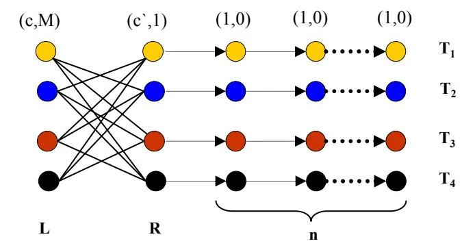
Figure 2: An illustration of a bidding problem with a large integrality gap (k = 3).

more important difference is the extra budget constraint. Because of this extra linear constraint, the following linear programming relaxation of this IP is not totally unimodular anymore.

$\begin{aligned} \text{Budgeted} - \text{LP} &: & \max \sum_{q_i \in Q} X_{q_i} v(q_i) n(q_i) \\ \text{For every pair } (q_j, q_i) \in \mathcal{C} &: & X_{q_i} - X_{q_j} \geq 0 \\ & & \sum_{q_i \in Q} X_{q_i} c(q_i) n(q_i) \leq B \\ \forall q_i \in Q &: & 0 \leq X_{q_i} \leq 1 \end{aligned}$

In fact, we can show that the integrality gap of this LP can be very large, and thus one cannot round the fractional solution of this linear programming relaxation to a good integral solution (as we did for IP 3.1).

Lemma 5.1. The integrality gap of linear programming relaxation 5.2 can be arbitrarily large.

PROOF. Consider the following instance of the bidding problem with a budget constraint in the query language: Let the set of queries $Q = R \cup L \cup T$ where $R = \{r_1, r_2, \dots, r_{k+1}\}$ , $L = \{l_1, l_2, \dots, l_{k+1}\}$ , and $T = T_1 \cup T_2 \cup \dots \cup T_{k+1}$ , where $T_i = \{t_{i1}, t_{i2}, \dots, t_{in}\}$ . For any query $q \in L$ , we have c(q) = c and v(q) = M, and for $q \in R$ , c(q) = c’ and v(q) = 1. We assume that c >> c’ >> n >> 1. For any $q \in T$ , v(q) = 0, and c(q) = 1. Also, let the query dependency structure be:

$\mathcal{C} = \{(r_i, l_j) | 1 \le i, j \le k+1, i \ne j\} \cup \{(r_i, t_{i1} | 1 \le i \le k+1\} \cup \{(t_{ij}, t_{i(j+1)} | 1 \le i \le k+1, 1 \le j \le n-1\}.$

It is easy to check that $\mathcal C$ matches the cost and query definitions. We also set the budget B=c+kc’+n. In this instance of the bidding problem, the optimal integer solution can pick at most one node from the set L (given the budget constraint of B and the fact that c>>c’>>n>>1), and thus the optimal integer solution is M+k.

On the other hand, as a fractional solution, we can set $x = \frac{(c+kc'+n)}{((k+1)c+(k+1)c'+n)}$ . The value of this fractional solution is $[(k+1)M+k+1]\frac{(c+kc'+n)}{((k+1)c+(k+1)c'+n)}$ which is approximately (k+1)M. As a result, the ratio between the optimal fraction solution and the integral solution can be as large as k. This proves that the integrality gap of the LP is arbitrarily large. $\square$

In fact, not only the LP for the budgeted problem is not integral, but also the optimal bidding problem with a budget constraint is an NP-hard problem even in the query language. The NP-hardness follows from the fact that this problem is harder than the knapsack problem. In fact, the knapsack problem is a special case of this problem in which the set of queries are only the keywords and $\mathcal{C} = \emptyset$ . Despite the large integrality gap of the above LP and NP-hardness of the problem, in the following we show how one can use a certain set of optimal solutions of this LP to implement two budget constrained ad campaigns for an ad auction with broad-match that achieves the optimal fractional solution of the above LP. We show this fact by proving the existence of optimal solutions for the LP with certain structural properties. The key structural lemma is the following:

Lemma 5.2. The Linear Program 5.2 has at least one optimal solution $X^*$ for which there exists a value X such that: for each query q, $X_q^* \in \{0, 1, X\}$ . Moreover, this optimal solution can be found in polynomial time.

PROOF. We prove this fact by showing that an optimal basic feasible solution of the LP satisfies the desired properties. From standard linear programming theory, we know that such a basic solution exists, and can be found in polynomial time. Consider an optimal basic feasible solution $X^*$ of the LP 5.2. Since the LP has |Q| variables, a basic feasible solution can be uniquely characterized by |Q| tight inequalities. In other words, there is a set P of |Q| independent linear equations among the linear constraints that characterize $X^*$ . Let $P_1 \subset P$ be a set of these |Q| linear equations of the form $X_{q_i}^* = 0$ or $X_{q_i}^* = 1$ . Each linear equation in $P_1$ corresponds to an integral variable $X_{q_i}^*$ . Let $S_1$ be the set of queries $q_i$ corresponding to these integral variables $X_{q_i}^*$ . Also let $P_2\subset P$ be a set of these |Q| linear equations of the form $X_{q_i}^*=X_{q_j}^*$ . We construct a graph $G(X^*, P_2)$ whose vertex set V(G) is the set of variables $X_{q_i}^*$ for all queries $q_i \in Q$ as follows: we put an edge between a vertex $X_{q_i}^*$ to a vertex $X_{q_j}^*$ if and only if $X_{q_i}^* = X_{q_j}^*$ is a linear equation in $P_2$ . Thus, if there is path between two nodes $X_{q_i}^*$ and $X_{q_j}^*$ in G, we have $X_{q_i}^* = X_{q_j}^*$ . Let the connected components of G be $G_1, G_2, \ldots, G_t$ . As a result, for any two variables $X_{q_i}^*$ and $X_{q_j}^*$ in the same connected component $G_p$ for $1 \leq p \leq t$ , we have $X_{q_i}^* = X_{q_i}^*$ (since there is a path between any two nodes in the same connected component.) We say that a connected component $G_p$ is a bad component if none of the nodes in $G_p$ are in $S_1$ . Otherwise, we say that $G_p$ is a good component. In the following, we show that the number of bad components is at most one, and this will prove the lemma. In order to prove this claim, we need to prove the following lemma:

LEMMA 5.3. Graph G as defined above does not have any cycle.

PROOF. For contradiction, assume that there exists a cycle $X_1^*, X_2^*, \cdots, X_v^*$ in graph G. Thus, all linear equations $X_i^* = X_{i+1}^*$ for $1 \leq i \leq v-1$ , and $X_v^* = X_1^*$ are in P. But these v equations are not independent, and this cycle contradicts the fact that P is a set of independent linear equations. $\square$

Lemma 5.3 proves that graph G is a forest, and thus connected components $G_i$ for $1 \le i \le p$ are all trees, and each

has $|V(G_i)| - 1$ edges. Now, we observe that for any good component $G_i$ , there exists exactly one equation in $P_1$ . For any good component $G_i$ , there are $|V(G_i)| - 1$ equations corresponding to edges of $G_i$ , and at least one equation in $P_1$ . If there two such equations in $P_1$ for nodes of $G_i$ , then the union of these two equations and equations corresponding to edges of $G_i$ form $|V(G_i)| + 1$ equations in P all defined on only variable on $V(G_i)$ . As a result, these equations cannot be independent, which contradicts with the fact that P is a set of independent equations. As a result, each good component $G_i$ corresponds to exactly $|V(G_i)|$ equations in P.

Let Y be the set of variables $X_{q_i}^*$ in good connected components of $G(X^*, P_2)$ . Thus, Y corresponds to a set of all integral variables $X_{q_i}^*$ . The above discussion implies that there are exactly $|Y|^{r}$ equations in P characterizing all variables in Y. As a result, there are |P|-|Y| equations uniquely identifying all the (fractional) variables in $Q \setminus Y$ . Noting that |P| = |Q|, we conclude that $|Q \setminus Y|$ equations uniquely identify all the (fractional) variables in $Q \setminus Y$ , and none of these equations are of the form $X_{q_i}^* = 0$ or $X_{q_i}^* = 1$ . At most one of these equations correspond to a tight budget constraint $(\sum_{q_i \in Q} X_{q_i}^* c(q_i) n(q_i) = B)$ , and thus we have at least $|Q\setminus Y|-1$ equations of the form $X_{q_i}^*=X_{q_i}^*$ on variables $Q \setminus Y$ in bad components. Since there is no cycle in graph G and vertices in $Q \setminus Y$ have at least $|Q \setminus Y| - 1$ edges amongst them, they should all belong to the same connected component (i.e, the only one bad connected component), and thus have the same value $X_{q_i}^* = X$ . This completes the proof of the lemma.

Using Lemma 5.2, we can show that in the query language model, one can implement the optimal fractional solution using two budget-constrained ad campaigns. To formally show this, we assume that queries arrive at the same rate, and by putting a budget constraint on an ad campaign (that includes a set of queries), the budget on all queries is consumed at the same rate until it gets used completely.

Theorem 5.4. In the query language model, there exists a polynomial-time algorithm that computes two budget-constrained ad campaigns that implement an optimal bidding strategy achieving the maximum value for the advertiser given a budget constraint.

PROOF. The polynomial-time algorithm is as follows:

• 1. Solve LP 5.2 and compute an optimal solution $X^*$ such that $X_{q_i}^* \in \{0, 1, X\}$ for all queries $q_i$ .
• 2. Let $S_0$ and $S_1$ be the sets of queries with the corresponding integral variables $X_{q_i}^* = 0$ and $X_{q_i}^* = 1$ , respectively.
• 3. Let $B_1 = \sum_{q_i \in S_1} X_{q_i}^* c(q_i) n(q_i)$ .
• 4. Run the following two ad campaigns:
  • (a) A campaign with budget $B_1$ on queries in $S_1$ .
  • (b) A campaign with budget $B B_1$ on queries in $Q \setminus (S_0 \cup S_1)$ .

Lemma 5.2 shows that the first step of this algorithm can be done in polynomial time. To show the correctness of the algorithm, note that assuming that queries arrive at the same rate, and based on the definition of the budgetconstrained ad campaign, the value from these two ad campaigns is:

$\sum_{q \in S_1} v(q)n(q) + \frac{B - B_1}{B'} \sum_{q \in Q \setminus (S_0 \cup S_1)} v(q)n(q),$

where $B' = \sum_{q \in Q \setminus (S_0 \cup S_1)} c(q) n(q)$ . Note that $X_{q_i}^* = 1$ for $q_i \in S_1$ , we have $B_1 = \sum_{q_i \in S_1} X_{q_i}^* c(q_i) n(q_i) = \sum_{q_i \in S_1} c(q_i) n(q_i)$ , and thus $B_1 + \sum_{q \in Q \setminus (S_0 \cup S_1)} X c(q) n(q) = B$ , therefore,

$X = \frac{B-B_1}{\sum_{q \in Q \backslash (S_0 \cup S_1)} c(q) n(q)} = \frac{B-B_1}{B'}.$

Thus, the value of the optimal solution is:

$\sum_{q \in S_1} v(q)n(q) + \sum_{q \in Q \setminus (S_0 \cup S_1)} Xv(q)n(q) =$ $\sum_{q \in S_1} v(q)n(q) + \frac{B - B_1}{B'} \sum_{q \in Q \setminus (S_0 \cup S_1)} v(q)n(q).$

Hence, the total value from these two campaigns is the same as the optimal fractional solution, as desired. $\Box$

Finally, we observe that the optimal bidding problem with a budget constraint is APX-hard for the keyword language.

Theorem 5.5. The optimal bidding problem with a budget constraint is APX-hard for the keyword language. Moreover, this problem is not approximable within a factor better than a multiplicative factor $1 - \frac{1}{\epsilon}$ .

PROOF. We give a simple reduction from the maximum coverage problem. In an instance of the maximum coverage problem, we are given a family of subset $S_1, \ldots, S_k \subset V$ , and a value w(e) for each element $e \in V$ . The goal is to find a family of k subsets $S_{a_1}, \ldots, S_{a_k}$ that maximizes $\sum_{e \in \cup_{i \le k} S_{a_i}}$ . Given an instance of the maximum coverage problem, we define an instance of optimal bidding problem as follows: for each subset $S_i$ $(1 \le i \le k)$ in the maximum coverage problem, we put a keyword $s_{S_i}$ in the set S of keywords in the optimal bidding problem. The cost c(s) of each keyword in S is 1 and its value is zero. We also put a query $q_e \in Q$ corresponding to each element $e \in V$ of the maximum coverage problem. The value of query $q_e \in Q \setminus S$ is one and the cost of each query is zero. Moreover, we say that a query $q_e$ corresponding to an element e can be broadly matched with any query $s_{S_i} \in S$ corresponding to any subset $S_i$ of the maximum coverage problem that includes the element e, i.e., $e \in S_i$ . Finally, we set the budget constraint B to k. It is not hard to see that the maximum value bidding strategy on keywords in this instance with the total cost at most B corresponds to the maximum value set-coverage of at most k sets in the original problem. This reduction implies that our problem is not approximable within a factor better than $1-\frac{1}{2}$ unless P=NP, since the maximum coverage problem is NP-hard to approximate within a factor better than $1 - \frac{1}{e} [8]$ .

6. AN EXPERIMENTAL STUDY

In this section, we report results from an experimental study to address how much an ad campaign loses by using solely broad match rather than a combination of exact and broad match types. Our simulation is composed of 30 keywords, where we consider all pairs of keywords as the set of possible queries. Therefore, while there are “only” 30 keywords an advertiser who is interested in managing all possible queries will have 435 keywords to consider, which is tedious for small advertisers. Most advertisers will prefer a campaign with a small set of keywords which they can easily track and evaluate, which in our simulation is represented by the core 30 keywords. The setup is very simple. All queries have the same cost. The net value of a query is determined as follows. The value of a keyword is drawn from a standard normal distribution. The net value of a query is either (1) the average net value of its keywords, or (2) the max value among its keywords, or (3) the min value among its keywords; the precise net value of a query is decided according to 1-3 uniformly at random. This setting is loosely motivated by the intuition that some queries just average the keywords in the query (like “Canon or Nikon”), some are valued as the best among the keywords (like “Canon DSLR”), and some valued as the worst among the keywords (like “Canon calculator”).

Running the simulation 15 times, we obtain that the average value obtained by solving the integer linear program while allowing both exact match and broad match was 120.9 while allowing only broad match was 119.2. Furthermore we obtain that the maximum ratio between the two was less than 4 percent. This simple simulation supports our initial hope that not using exact match may be a realistic assumption for some advertisers, in particular, small to medium advertisers. We must remark that a more detailed experimental study is needed to be more conclusive. Our hope is that our LP-based algorithms can indeed be run with reasonably sized problems for this purpose.

7. CONCLUDING REMARKS

Our work initiates the study of the bid optimization problem for advertisers in presence of a common feature in sponsored search, ie., the broad match type. The central technical issue is that choosing to bid on a keyphrase may yield positive profit from some queries, but may commit one to implicitly bid on queries in which the profit may be small or even negative. We propose LP-based polynomial-time algorithms for this problem which is optimal under the query language model, and is an approximation in the keyword language model for certain cases while it is NP-Hard to even approximate the optimal solution to any factor, in general.

Our work leaves open several research problems. A technical problem is to extend the results here to the multi-slot case. More precisely, given a “landscape” that is a function of bids and gives estimated clicks and cost, obtain the profit-maximizing bidding strategy. A conceptual problem is to determine a suitable approach for broad match auctions where search engines are able to provide faithful estimates for clicks and cost associated with the broad matches, so advertisers can bid accurately. This involves averaging over many related queries. A principled approach to formulating this notion will be of great interest.

Finally, a specific technical question that remains open in this paper is the approximability of the budget-constrained version of the optimal bidding problem in the keyword language. An interesting aspect of this problem is the following relation to submodular optimization. Given a subset $T \subset S$ of keywords on which we can bid, let us denote the total cost

and value of the queries that we win as a result of bidding on keywords in T by C(T ) and V (T ). One can check that both the value and cost functions V, C : 2^S → R are setcover-type set functions, and thus they are monotone and submodular. 5 The optimal bidding problem with a budget constraint in the query language is, therefore, to find a subset T ⊂ S of keywords that maximizes the submodular function V (T ) subject to the submodular constraint C(T ) ≤ B. Constant-factor approximation algorithms are known for maximizing a general monotone submodular function subject to a knapsack (modular) constraint [19], but maximizing submodular functions subject to a submodular constraint (as in our case) is an open question.

8. REFERENCES

• [1] Position Auctions with Consumer Search. Working Paper, Sept 2007.

• [2] G. Aggarwal, A. Goel, and R. Motwani. Truthful auctions for pricing search keywords. In ACM Conference on Electronic Commerce (EC), 2006.

• [3] G. Aggarwal and J. D. Hartline, Knapsack Auctions, Proceedings of the Seventeenth Annual ACM-SIAM Symposium on Discrete Algorithms (SODA), 2006.

• [4] C. Borgs, J. Chayes, O. Etesami, N. Immorlica, K. Jain, M. Mahdian: Dynamics of bid optimization in online advertisement auctions. WWW 2007: 531-540

• [5] C. Borgs, J. T. Chayes, N. Immorlica, M. Mahdian, and A. Saberi. Multi-unit auctions with budget-constrained bidders. In ACM Conference on Electronic Commerce (EC), 2005.

• [6] D. Chakrabarty, Y. Zhou, R. Lukose. Budget Constrained Bidding in Keyword Auctions and Online Knapsack Problems. 3rd Workshop on Sponsored Search Auctions (SSA), 2007.

• [7] B. Edelman, M. Ostrovsky, and M. Schwarz. Internet advertising and the generalized second price auction: Selling billions of dollars worth of keywords. In Second workshop on sponsored search auctions, 2006.

• [8] U. Feige. A Threshold of ln n for Approximating Set Cover. Journal of ACM, 45(4):634-652, 1998

• [9] J. Feldman, S. Muthukrishnan, M. P´al and C. Stein. Budget optimization in search-based advertising auctions. ACM Conference on Electronic Commerce, 2006.

• [10] M. Garey and D. Johnson. Computers and Intractability: A Guide to the Theory of NP-Completeness. WH Freeman & Co New York, 1979.

• [11] D. Martin, J. Gehrke, and J. Halperin. Toward Expressive and Scalable Sponsored Search Auctions http://www.cs.cornell.edu/johannes/papers/2008/icde2008-auctions.pdf

• [12] M. Mahdian, H. Nazerzadeh, and A. Saberi Allocating Online Advertisement Space with Unreliable Estimates Proceedings 8th ACM Conference on Electronic Commerce (EC), 2007.

• [13] A. Mehta, A. Saberi, U. Vazirani, and V. Vazirani. AdWords and Generalized Online Matching. Journal of the ACM, Volume 54 , Issue 5, 2007.

• ⁵A set function f : 2^S → R is submodular if and only for any two subsets A and B, f(A) + f(B) ≥ f(A ∩ B) + f(A ∪ B).

• [14] S. Muthukrishnan, M. P´al, and Z. Svitkina. Stochastic models for budget optimization in search-based advertising. In Proc. Workshop on Internet and Network Economics (WINE), 2007.

• [15] Christos H. Papadimitriou and Kenneth Steiglitz. Combinatorial Optimization. Prentice Hall

• [16] P. Rusmevichientong and D. Williamson. An adaptive algorithm for selecting profitable keywords for search-based advertising services. ACM Conference on Electronic Commerce 2006: 260-269.

• [17] A. Schrijver. Combinatorial Optimization. Springer, 2003.

• [18] M. Stoer and F. Wagner. A simple min-cut algorithm. Journal of the ACM, 44(4):585-591, July 1997.

• [19] M. Sviridenko. A note on maximizing a submodular set function subject to knapsack constraint. Operations Research Letters 32 (2004), 41–43.

• [20] H. Varian. Position auctions. International Journal of Industrial Organization, 25(6):1163–1178, December 2007.

• [21] http://adcentercommunity.com/blogs/advertiser/archive/2008/04/07/keyword-match-types.aspx.

• [22] http://help.yahoo.com/l/us/yahoo/ysm/sps/start/overview\_matchtypes.html.

• [23] http://adwords.google.com/support/bin/answer.py?hl=en&answer=6100.

• [24] http://adwords.google.com/support/bin/answer.py?answer=25148.

• [25] http://sem.smallbusiness.yahoo.com/searchenginemarketing/index.php?&abr=2022403519.

• [26] https://adcenter.microsoft.com/Default.aspx.

• [27] Yahoo! Search Marketing Advertiser Workbook http://us.i1.yimg.com/us.yimg.com/i/us/ysm/misc/pdf/eworkbook.pdf

• [28] https://clients.mamma.com/faq/bidsystem/faq\_broad\_matching.html.