Estimating Individual Advertising Effect In E Commerce

Abstract

Online advertising has been the major monetization approach for Internet companies. Advertisers invest budgets to bid for real-time impressions to gain direct and indirect returns. Existing works have been concentrating on optimizing direct returns brought by advertising traffic. However, indirect returns induced by advertising traffic such as influencing the online organic traffic and offline mouth-to-mouth marketing provide extra significant motivation to advertisers. Modeling and quantization of causal effects between the overall advertising return and budget enable the advertisers to spend their money more judiciously. In this paper, we model the overall return as individual advertising effect in causal inference with multiple treatments and bound the expected estimation error with learnable factual loss and distance of treatmentspecific context distributions. Accordingly, a representation and hypothesis network is used to minimize the loss bound. We apply the learned causal effect in the online bidding engine of an industrylevel sponsored search system. Online experiments show that the causal inference based bidding outperforms the existing online bidding algorithm.

1 Introduction

The last two decades have seen the prosperity of e-commerce. Taking Taobao as an example, as the biggest e-commerce marketplace in China [Edquid, 2016], Taobao search service covers over 300 million consumers each day, bringing daily 10 billion search queries and subsequent page views (PVs), providing advertisers sufficient opportunities to promote their commodities online ¹.

In sponsored search advertising, advertisers bid for keywords associated with their commodities (ADs ²) and pay the platform when consumers land their commodity/store homepage by clicking the advertisement (Pay-Per-Click,

PPC). The payment equals the minimum bid price required to keep the advertising slot in the real-time competition [Wilkens et al., 2017]. The returns of advertising can be summarized in two aspects. The direct returns of advertising are the impressions, clicks and conversions occurred upon the advertising PVs. Meanwhile, advertising also yields even more valuable indirect returns by connecting with wider online audience, thus impressing more audience via unobserved social interactions. Additionally, in e-commerce platform like Taobao, there is a ranking index called “sales volume” for organic search traffics, which reflects the purchasing popularity of the commodity among its peers and has been an important shopping guideline for consumers. In this way advertisers can accumulate sales volume via advertising PVs to gain more exposures in gigantic organic search PVs.

The direct and indirect returns motivate advertisers to invest advertising budget to prosper their online business. Despite its significance, however, to the best of our knowledge, existing work mostly focus on optimizing direct returns [Zhang, 2016; Zhu et al., 2017]. This might be caused by the fact that direct returns are seamlessly observable in the closed-loop e-commercial platform like Taobao. Meanwhile, there are so many factors leading to the overall returns, making it intractable to quantify the indirect returns attributed to advertising. Nonetheless, the ability of inferring the overall advertising effect including both direct and indirect returns provide advertisers the opportunities to allocate their advertising budget more wisely in the product life cycle.

E-commercial advertisers are eager to know the growth of advertising returns if they invest more budget via a specified advertising channel. Specifically, in the PPC advertising, the cost is equivalent to the number of clicks occurred in advertising PVs given a relatively stable payment per click. And the overall advertising returns can be observed as the number of total clicks of the advertising AD accumulated in all the online channels. Therefore, we want to infer the individual advertising effect (IAE) via predicting the incremental number of all-channel clicks in a period under the intervention of advertising clicks ³.

^<sup>2A commodity is also called an AD in Taobao, which represents both the commodity and the associated advertisement.

^<sup>3Numerical analysis also shows that the Pearson’s coefficient between the number of advertising clicks and all-channel clicks is approximately 25% larger than that between advertising impressions and all-channel clicks. We hide the detailed coefficient value due to commercial secrets.

The problem of inferring IAE resembles the estimation of individual treatment effect (ITE) in the field of causal inference or learning from observational data [Rubin, 2005]. In causal inference, we only have observational data which contains the past actions, their outcomes and possibly more context. However, we do not know the mechanism which gave rise to the action. In the scenario of advertising, the context might correspond to the features representing the current status of the AD, while the action and outcome are the number of advertising clicks and all-channel clicks (containing all direct and direct returns), respectively. The key difference between IAE and ITE is that actions of the latter are binary or categorical, but those of the former might be continuous and transitive. Furthermore, for any specified context, there exists only one exact action (acquire specific number of advertising clicks) in the data. We can never know exactly the potential advertising outcome if it applies a different action in exactly the same context. Besides, the observed advertising outcomes can be influenced by a lot of factors including online sources such as in or out of Taobao recommendation/organic search, and offline mouth-to-mouth marketing by the audience etc, which is similar to the confounding factor in classic causal inference. Since the effect of advertising is accumulating in the whole-time horizon, we assume that the context together with the action contain all the necessary information to determine the outcome, i.e., the “no-hidden confounding” assumption holds in the analysis.

In this paper we model the causal effect between advertising cost and returns via a formal definition of IAE. We propose a representation network and a hypothesis network combined to predict the individual advertising effect referring [Shalit et al., 2017]. Different from binary or categorical treatments, advertising treatments are continuous and transitive. Relying on this property, we derive a rigorous theoretical upper bound of the expected IAE estimation error by way of a learnable factual regression loss and the distance of context distribution among different treatments. Then the network is trained to minimize the derived theoretical upper bound. Furthermore, we derive a time-varying factor called leverage rate (lvr) based on IAE to reflect the AD-level potential to lever the overall advertising returns. The learned lvr is used in the online bidding engine to achieve better overall advertising performance in Taobao sponsored search. The contributions of this paper can be summarized as follows:

• 1. We model the problem of predicting the overall advertising return in the framework of causal inference. In this framework, the formal definition of individual advertising effect is given.
• 2. We derive a general theoretical upper bound on the expected IAE estimation error in advertising scenarios with multiple continuous and transitive treatments. Subsequently, a representation and hypothesis network is learned to predict IAE.
• 3. IAE-induced lvr is integrated in the online bidding engine, which yields better overall advertising returns compared with the existing bidding engine in Taobao sponsored search.

2 Related Work

When considering only direct advertising returns, estimating individual advertising effect has been investigated in both ex ante and ex post way. The key of the ex ante estimation lies in three separate models of predicting the winning rate of specific bids, click-through-rate and conversionrate of the advertising PV [Zhang, 2016; Zhu et al., 2017]. Meanwhile, attribution modeling [Dalessandro et al., 2012; Diemert et al., 2017] corresponds to the ex post estimation of advertising effect, i.e. attributing the later conversion to the previous customer-commodity/store contact. All these works ignore the indirect returns brought by the advertising PVs.

Causal inference has already been used in complex realworld ad-placement systems [Bottou et al., 2013]. In the scenario of estimating individual advertising effect, given a context (AD), a naive way might be direct least square regression to fit the advertising effect, either taking the number of advertising clicks as a feature or separately fit each action. However, such estimation might be biased due to the fact that different contexts should have priority of choosing specific actions in the dataset. To alleviate the bias, propensity score, which characterizes the probability vector of choosing specific actions, [Austin, 2011] is used to evaluate the similarity of two contexts. Therefore, counterfactual samples can be constructed by comparing the propensity scores via various approaches such as nearest neighbor matching [Lopez et al., 2017]. Besides propensity score, various methods such as random forests[Wager and Athey, 2017; Athey and Imbens, 2016] and expensive random control trials [Taddy et al., 2016; Peysakhovich and Lada, 2016] are also used to tackle the binary treatment causal inference.

Recently deep representation is also used to encode the contexts. Atan et al. proposed an auto encoder-decoder network to represent the raw context, to ensure that the propensity score vector of the mapped contexts is similar, therefore removing the selection bias [Atan et al., 2018]. Johansson et al. also designed a deep representation network to embed the original contexts, to guarantee that the distribution of contexts after the representation is similar between two different treatments, as well as the small regression loss [Johansson et al., 2016]. In its later version, a theoretical error bound on the expected ITE is given to yield a more rigorous estimation algorithm [Shalit et al., 2017]. Deep models prove to be advanced but when faced with the multiple treatments, theoretical error bound is non-trivial. In this paper we design a similar network structure as [Shalit et al., 2017] but derive our theoretical upper bound considering the continuous action space in the advertising scenario.

Back to the bidding application, perhaps the most relevant work is lift-based bidding proposed by Xu et al. By predicting the ex ante and ex post click-through-rate of an advertising impression, the bid price is adjusted to be proportional to the lift [Xu et al., 2016]. However, we point out that the observed outcome might also ignore the abundant indirect returns.

3 Individual Advertising Effect Formalization

We adopt the Rubin-Neyman potential outcomes modeling framework [Rubin, 2005] in causal inference but tailor it for the e-commerce advertising scenario. Let $\mathcal{X} \subset \mathbb{R}^d$ be the set of contexts, $\mathcal{T} = \{T_1,...,T_n\}$ the n-action (also known as treatment or intervention) set, $\mathcal{Y} \subset \mathbb{R}$ the observed overall performance index. For each context $x \in \mathcal{X}$ , there is a treatment assignment $T \in \mathcal{T}$ and with n potential outcomes, $Y_{T_1}, Y_{T_2}, ..., Y_{T_n} \in \mathcal{Y}$ . The samples we have can be denoted as $\{x_i, t_i, y_i\}_{i=1}^N$ , where $y_i = Y_{t_i}$ . We do not observe any of the other potential outcomes (i.e., $Y_T$ for $T \neq t_i$ ).

In e-commercial advertising, context x can be features representing the status of an AD in the beginning of the day. Treatment T refers to the number of clicks acquired from the advertising PVs during the day, while potential outcome y might be observed as the overall whole-site clicks obtained by the same AD until the end of the day. Apparently, the potential outcome can be influenced by a lot of factors including online channels such as in or out of Taobao recommendation/organic search, and offline mouth-to-mouth marketing by extroverted audience etc. Specifically, let $T_i = i - 1, i = i - 1$ 1, …, n, where n-1 can be interpreted as the context-specific largest possible advertising clicks in a day. Note that we restrict the advertising effects y to be happened in the same day, but ignores the persisting effects in the far future. This naturally coincides with the advertising logic that advertisers are accustomed to adjusting the budget of an AD day by day. We can also alleviate the influence of persisting dependency by following the “strong ignorability” assumption in causal inference.

Assumption 1. (Strong Ignorability) $Y_{T_1}, Y_{T_2}, ..., Y_{T_n} \perp T | x$ , which means that, given a context x, the potential outcome is independent of the treatment assignment.

Strong ignorability assumption also ensures that there is a positive probability of choosing any action in each context x.

Definition 1. (Individual Advertising Effect, IAE) The IAE of context x from treatment $T_i$ to $T_j$ can be defined as:

$\alpha_{i,j}(x) = m_j(x) - m_i(x), \forall i, j = 1, ..., n,$ (1)

where $m_i(x) = \mathbb{E}[Y_{T_i}|x], \forall i, j = 1, ..., n$ .

For n treatments, we can obtain an antisymmetric matrix $\alpha(x) = [\alpha_{i,j}] \subset \mathbb{R}^{n \times n}$ which corresponds to the IAE in context x. Matrix $\alpha(x)$ has the following properties:

• Antisymmetric: $\alpha_{i,j} = -\alpha_{j,i}$ ;
• Monotonicity: $\alpha_{i,j} \leq \alpha_{i,k}, \forall j \leq k, i = 1, ..., n; \alpha_{i,j} \geq \alpha_{k,j}, \forall i \leq k, j = 1, ..., n;$
• Zero-Diagonal: $\alpha_{i,i} = 0, \forall i = 1,..,n;$
• Transitivity: $\alpha_{i,j} + \alpha_{j,k} = \alpha_{i,k}, \forall i, j, k = 1, ..., n$ .

In causal inference, IAE is analogous to individual treatment effect. However, different from classical causal inference with only two interventions of either treatment or nontreatment, multiple actions are available in IAE. Since the action and outcome are accumulated in a day, there is some kind of ambiguity of advertising effect with clicks assigned to different time slots. Therefore, we take the expectation in the

right-hand side of Eqn. (1) to eliminate the ambiguity. In this sense, IAE is the average advertising effect and should be useful among different ADs.

To learn IAE, we further define a representation function $\Phi: \mathcal{X} \to \mathcal{R}$ where $\mathcal{R}$ is the representation space. Let $h: \mathcal{R} \times \mathcal{T} \to \mathcal{Y}$ be a hypothesis function which yields the outcome. Putting it together, we denote $f(x,T) = h(\Phi(x),T)$ .

Definition 2. Given a hypothesis f, the IAE estimation for context x is:

\hat{\alpha}_{i,j}^{f}(x) = f(x, T_j) - f(x, T_i). \tag{2}

With a little abuse of notation, we will omit the superscript f and write it as $\hat{\alpha}_{i,j}(x)$ without confusion.

Definition 3. The IAE estimation error of treatment pairs $(T_i, T_j)$ satisfies that:

\tau_{i,j}(x) = \hat{\alpha}_{i,j}(x) - \alpha_{i,j}(x). \tag{3}

Definition 4. The expected Precision in Estimation of Heterogeneous Effect (PEHE) [Shalit et al., 2017] loss of f is:

$\epsilon_{PEHE}(f) = \frac{1}{n(n-1)} \sum_{i=1}^{n} \sum_{j=1, j \neq i}^{n} \int_{\mathcal{X}} \tau_{i,j}^{2}(x) p(x) dx.$ (4)

For completeness, we also give the notion of Integral Probability Metric (IPM), which is a class of distance metrics between probability distributions [Shalit et al., 2017]. For two probability density functions p, q defined over $S \subset \mathbb{R}^d$ , and for a function family G as $g: S \to \mathbb{R}$ , it holds that

$IPM_G(p,q) := \sup_{g \in G} |\int_{\mathcal{S}} g(s)(p(s) - q(s))ds|.$

4 Learning to Infer Individual Advertising Effect

The key of learning IAE lies in minimizing the PEHE loss in Eqn. (4). The idea is similar as [Shalit et~al., 2017]. Firstly, we map the original context into the representation space $\mathcal R$ via $\Phi$ . In the new space, we denote the probability density function of representation space $\mathcal R$ given treatment T as $p_{\Phi}^T$ . To remove the selection bias in the original space, the idea is that the distance between $\{p_{\Phi}^{T_i}\}_{i=1}^n$ should be as small as possible, which is guaranteed by the representation network. Given the similar context distribution in the representation space, the hypothesis network should try to minimize the regression loss of fitting the advertising return. The neural network architecture is displayed in Fig. 1.

The architecture resembles that in [Shalit et al., 2017]. However, the key differences lies in two aspects. Firstly, the hypothesis network in that of [Shalit et al., 2017] are separate for treatment/non-treatment. In the advertising scenario, the treatments can be seen as continuous actions and should be generalizable, therefore different treatments share the same hypothesis network. Secondly, IPM for binary treatments are straightforward while it is not obvious for multiple treatments. We simplify the IPM term based on the transitive property of treatment effects. In the following part we will first give the theoretical upper error bound of PEHE error and elaborate the detailed IPM we use, followed by the description of the IAE estimation algorithm.

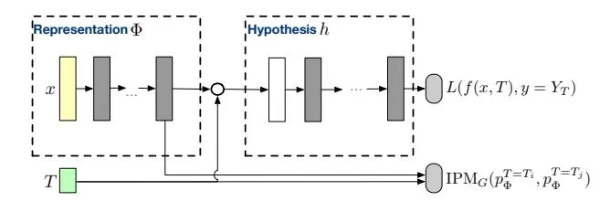
Figure 1: Neural network architecture for IAE estimation. L is a loss function and $\Phi$ is a representation of the original context x. h represents the hypothesis and f denotes the complete function.

4.1 Loss Error bound

Before analyzing our main result, we first give a lemma considering the binary treatment case.

Lemma 1. [Shalit et al., 2017] Let $\Phi: \mathcal{X} \to \mathcal{R}$ be a one-to-one representation function with inverse $\Psi$ . Let $h: \mathcal{R} \times \{T_i, T_j\} \to \mathcal{Y}$ be an hypothesis. Assume there exists a constant $B_{\Phi}$ such that for $T \in \{T_i, T_j\}$ , the per-unit expected loss functions $\ell_{h,\Phi}(\Psi(r),T)$ obey $\frac{1}{B_{\Phi}} \cdot \ell_{h,\Phi}(\Psi(r),T) \in G$ , where $\ell_{h,\Phi}(x,T) = \int_{\mathcal{Y}} L(h(\Phi(x),T),Y_T)p(Y_T|x)dY_T$ . Assuming that the loss L is the squared loss, we have that

2(\epsilon_{F}^{T=T_{i}}(h, \Phi) + \epsilon_{F}^{T=T_{j}}(h, \Phi) + B_{\Phi} IPM_{G}(p_{\Phi}^{T=T_{i}}, p_{\Phi}^{T=T_{j}})),$$ where we omit the term of minus variance in the righthand side. And $\epsilon_F^T(h,\Phi) = \int_{\mathcal{X}} \ell_{h,\Phi}(x,T) p^T(x) dx$ , which represents the learnable factual loss of treatment T. In the binary case, Shalit *et al.* separate the regression loss of treatment/non-treatment for the categorical treatments. In our scenario, the treatments are continuous advertising clicks and should be generalizable across different treatments. In this case we define the regression loss with respect to treatments $\{T_i, T_j\}$ as <span id="page-3-3"></span> $$\epsilon_{i,j}(h,\Phi) = \epsilon_F^{T=T_i}(h,\Phi) + \epsilon_F^{T=T_j}(h,\Phi).$$ (5) Then we are ready to decompose the PEHE error. <span id="page-3-2"></span>**Lemma 2.** In the continuous and transitive treatments scenario, it satisfies that $$\epsilon_{PEHE}(f) \le \sum_{i=1}^{n-1} \int_{\mathcal{X}} \tau_{i,i+1}^2(x) p(x) dx. \tag{6}$$ *Proof.* It follows that: $$\begin{split} \tau_{i,j}(x) &= \hat{\alpha}_{i,j}(x) - \alpha_{i,j}(x) \\ &= f(x,T_j) - f(x,T_i) - m_j(x) + m_i(x) \\ &= f(x,T_j) - f(x,T_{j-1}) + f(x,T_{j-1}) - f(x,T_{j-2}) \\ &+ \dots + f(x,T_{i+1}) - f(x,T_i) \\ &- m_j(x) + m_{j-1}(x) - \dots - m_{i+1}(x) + m_i(x) \\ &= \hat{\alpha}_{j-1,j}(x) + \dots + \hat{\alpha}_{i,i+1}(x) \\ &- \alpha_{j-1,j}(x) - \dots - \alpha_{i,i+1}(x) \\ &= \tau_{i,i+1}(x) + \tau_{i+1,i+2}(x) + \dots + \tau_{j-1,j}(x) \end{split}$$ Therefore, according to the Cauchy-Schwarz inequality, we have that $$\tau_{i,j}^2(x) \le (j-i)[\tau_{i,i+1}^2(x) + \dots + \tau_{j-1,j}^2(x)], \forall j > i.$$ Apparently, $\tau_{i,j}(x) = -\tau_{j,i}(x)$ . Then the PEHE loss can then be written as: $$\begin{split} \epsilon_{\text{PEHE}}(f) &\leq \frac{2}{n(n-1)} \sum_{i=1}^n \sum_{j>i}^n \int_{\mathcal{X}} \tau_{i,j}^2(x) p(x) dx \\ &= \sum_{i=1}^{n-1} \int_{\mathcal{X}} \tau_{i,i+1}^2(x) p(x) dx. \end{split}$$ Combining Lemma 1, Lemma 2 and Eqn. (5), we obtain a learnable upper bound for PEHE. <span id="page-3-4"></span>**Theorem 1.** Under the assumptions in Lemma 1 and Lemma 2, we have that: $$\epsilon_{PEHE}(f) \le 2 \sum_{i=1}^{n-1} \left[ \epsilon_{i,i+1}(h, \Phi) + B_{\Phi} IPM_G(p_{\Phi}^{T=T_i}, p_{\Phi}^{T=T_{i+1}}) \right].$$ (7) Theorem 1 directly points out an algorithm for learning IAE. Relying on continuous and transitive treatments, it generalizes the binary treatments to the multiple treatments advertising scenario. Note that we can compare arbitrary pairwise treatment effect via customized definition of PEHE loss. #### 4.2 Algorithm implementation In the advertising data, the context x mainly embeds the status of an AD with its features in major traffic channels. In our case, we choose the following features to characterize an AD before applying treatment T: - IDs: including the commodity ID, the shop ID, the category ID and other one-hot encoding features such as weekdays/weekends etc; - PV sources of the AD in the last day: we aggregate the advertising effects from the major online PV sources of the last day, mainly including sponsored search, recommendations, organic search, etc. Moreover, we also include the time when the AD was created and shelved; - PV sources of the AD in the last week: the exponential decaying average advertising effects of last week, including major online PV sources as the above one; - Shop features: including the number of impressions and clicks of the shop in the last day. Moreover, the count of total clicks of the shop, the total number of ADs and also the ADs in sponsored search advertising campaign of the shop are also included; - Competition of the last day: the average ranking of the AD and shop in the bidding process of the last day, with the logarithm of the two values included. We believe the above features cover most of the data we can fetch online for an AD in Taobao platform. We learn to infer IAE by minimizing the upper bound of the nominal PEHE loss, using the following objective: <span id="page-4-0"></span> $$\begin{split} \min_{h,\Phi} \quad & \frac{2}{N} \sum_{i=1}^N w_i \cdot L(h(\Phi(x_i),t_i),y_i) + \lambda \cdot \mathscr{R}(h) \\ & - \frac{\mu_1}{N} \cdot \sum_{i=1}^N L(h(\Phi(x_i),t_i),y_i) \mathbf{1}_{t_i = T_1} \\ & - \frac{\mu_n}{N} \cdot \sum_{i=1}^N L(h(\Phi(x_i),t_i),y_i) \mathbf{1}_{t_i = T_n} \\ & + \beta \cdot \sum_{i=1}^{n-1} \mathrm{IPM}_G(p_\Phi^{T=T_i},p_\Phi^{T=T_{i+1}}), \end{split}$$ with $\mu_j = \frac{N_j}{N}, w_i = \mu_{t_i}, N_j = \sum_{i=1}^N \mathbf{1}_{T_j = t_i}, j = 1, ..., n, \end{split}$ and $\mathcal{R}$ is a model complexity term. Note that $w_j, j = 1, ..., n$ corresponds to the proportion of units applying treatment $T_i$ in the whole population, which is approximated by the sample population. And $\mathbf{1}_{condition}$ is an indicator function which yields 1 when the condition is true; otherwise 0. We use the same $B_{\Phi} = \beta$ across all the IPM distance since they have the same importance in the PEHE definition. We train the models by using stochastic gradient descent to minimize (8) with $\ell_2$ -regularization and 1-Lipschitz function family G. Samples belonging to different treatments share a common representation and hypothesis as shown in Fig. 1. The details of the training process is shown in Algorithm 1. The algorithm structure is much like that in [Shalit et al., 2017] with differences on objective function and gradients. We put it here for completeness. ## **Causal Inference Based Bidding** Real-time bidding has been investigated thoroughly in recent years [Zhu et al., 2017; Perlich et al., 2012; Zhang et al., 2014]. For e-commercial advertisers in pursuit of conversions, the optimal bidding algorithms share a common value-based form as: $$bid = \gamma * cvr * ip, \tag{9}$$ where cvr, ip are the predicted conversion rate and item price, respectively. $\gamma$ is a used to regulate the return-on-investment (ROI)/budget of the advertiser. Larger $\gamma$ leads to lower ROI but obtains more impressions. In Taobao sponsored search practice, $\gamma$ is interpreted as the inverse of the expected ROI of the advertiser, which can be estimated from the historical auction log and advertiser's keyword-level bid settings. Apparently, the above bidding only considers the promotion value induced by the advertising PVs, i.e., the direct returns. To bid for the overall returns, we define an AD-level *leverage* rate (lvr) based on IAE. **Definition 5.** The leverage rate for context x with advertising *clicks changing from s to t is:* $$\sigma_{s,t}(x) = \frac{\hat{\alpha}_{s,t}(x)}{t-s}.$$ (10) ## <span id="page-4-1"></span>Algorithm 1 Learning Individual Advertising Effect **Input:** Samples $\{(x_i, t_i, y_i)\}_{i=1}^N$ , loss function $L(\cdot)$ , regularization factor $\lambda$ and $\beta$ , representation network $\Phi_{\mathbf{W}}$ with initial weights W, hypothesis network $h_V$ with initial weights, function family G for IPM distance, regulariza- Output: Representation and hypothesis network. **Dutput:** Representation and hypothesis network. Compute $$N_j = \sum_{i=1}^N \mathbf{1}_{T_j=t_i}$$ Compute $\mu_j = \frac{N_j}{N}, w_i = \mu_{t_i}$ while not converged **do** Sample mini-batch $i_1, i_2, ..., i_l \subset \{1, 2, ..., N\}$ Calculate the gradient of the IPM sum term: $g_1 = \nabla_{\mathbf{W}} \sum_{i=1}^{n-1} \mathrm{IPM}_G(p_{\Phi}^{T=T_i}, p_{\Phi}^{T=T_{i+1}})$ Calculate the gradients of the empirical loss: $g_2 = \nabla_{\mathbf{V}} L, g_3 = \nabla_{\mathbf{W}} L$ where $L = \frac{2}{m} \sum_j w_{i_j} \cdot L(h(\Phi(x_{i_j}), t_{i_j}), y_{i_j})$ where $L = \frac{N}{m} \cdot \sum_{i=1}^{N} L(h(\Phi(x_{i_j}), t_{i_j}), y_{i_j}) \mathbf{1}_{t_{i_j} = T_1} - \frac{\mu_n}{m} \cdot \sum_{i=1}^{N} L(h(\Phi(x_{i_j}), t_{i_j}), y_{i_j}) \mathbf{1}_{t_{i_j} = T_n}$ Calculate step size scalar or matrix $\eta$ with Adam [Kingma and Ba, 2014] $[\mathbf{W}, \mathbf{V}] \leftarrow [\mathbf{W} - \eta(\beta g_1 + g_3), \mathbf{V} - \eta(g_2 + 2\lambda \mathbf{V})]$ Check convergence condition lvr reflects the average number of all-channel clicks obtained per advertising click invested. Apparently, in the perspective of an AD, lvr is changing as time evolves, which might be influenced by the shifting marketing environment. In the slowly drifting bidding environment, the number of advertising clicks an AD can obtain might also gradually change, which gives an opportunity for the AD to take full advantage of the change. In this sense, lvr can also be seen as the partial derivative of the overall clicks with respect to the advertising clicks. Specifically, for an AD in context x, we define the nominal lvr by taking s and t to be the most recent daily advertising clicks obtained by the same AD. For example, let t be the number of advertising clicks obtained by the same AD yesterday while s corresponds to that obtained the most recent day other than yesterday, satisfying $s \neq t$ . Then the AD-level nominal lvr for today is $\sigma$ . We incorporate the nominal lvr in the bidding equation as: end while <span id="page-4-2"></span> $$bid = \sigma * \gamma * cvr * ip. \tag{11}$$ In light of lvr, the bidding takes into account the average overall return including both clicks from advertising PV itself and the indirect clicks caused by the advertising effect. In the bidding process, the new bidding formula as in Eqn. (11) should allocate more budget to those with the potential to leverage more all-channel clicks. The overall returns of advertising should be improved given the same budget. ## **6** Online Experiments Different from classical machine learning tasks, to evaluate causal effect is intractable due to the missing counterfactual outcomes in reality. Existing binary-treatment work relies on synthetic or simulated dataset such as IHDP and Jobs [Yao et al., 2018] to evaluate. For multiple treatment scenario, to the best of our knowledge, there only exists a multiple intervention breast cancer dataset [Yoon et al., 2017], which is not public however. To this end, we turn to evaluate the causal effect estimation by applying it to the online bidding engine in Taobao sponsored search, to compare the bidding performance with the existing online bidding algorithm, which has already been proved to be a strong baseline in practice. In Taobao sponsored search system, we randomly choose a set of ADs $\mathcal{A}$ to carry out the experiment. The nominal lvr distribution in $\mathcal{A}$ is similar with that in the whole set. We apply the lvr-induced bidding for ADs in $\mathcal{A}$ and keep the remaining as the control group. For AD $a_i \in \mathcal{A}$ , the bidding equation is: $$bid_i = \kappa * \frac{\sigma_i}{\bar{\sigma}} * \gamma * cvr * ip, \forall a_i \in \mathcal{A}, \bar{\sigma} = \frac{\sum_i \sigma_i}{|\mathcal{A}|}$$ where $\sigma_i$ corresponds to the nominal lvr of AD $a_i$ and $|\mathcal{A}|$ is the cardinality of $\mathcal{A}$ . Furthermore, $\kappa$ is utilized to adjust the bidding formula to ensure that the total advertising cost of all the ADs in $\mathcal{A}$ is approximately the same with that applying the existing bidding equation. $\kappa$ is updated daily by an offline replay system and applied online in the new day. The replay system evaluates the cost with respect to bidding given the daily auction log. Note that the same advertising cost implies that the number of advertising clicks is also nearly the same. We compare the number of all-channel clicks obtained in the lvr-bidding group, with those of the control group as the baseline. Specifically, we separately show the number of clicks obtained in Taobao organic search engine, which is the major source of free clicks. For commercial secrets, we hide the absolute value but show the relative incremental ratio based on the control group. We display the relative incremental ratio of number of advertising clicks (Ad)/all-channel clicks (All)/organic search clicks (Search) of the lvr-bidding group in Fig. 2. The lvr-bidding goes online on Dec. 23, 2018 and offline at the end of Dec. 28, 2018 (included). It can be seen that as the lvr-bidding goes online, although the number of advertising clicks goes down 2 percent, the number of allchannel clicks obtained by the same ADs sees an increase of 2 percent, while the number of organic search clicks increases 4 percent, which is significant improvement in a giant system like Taobao sponsored search. Furthermore, the ratio of all-channel clicks/organic search clicks over advertising clicks also experiences nearly the same increase pattern. The contradicted variation between advertising and performance here means that advertisers actually improve their marketing performance even with less investments via allocating budgets based on causal effects. As the lvr-bidding goes offline, the performance resembles that before the experiment, which shows a relative stable marketing environment during the whole period. <span id="page-5-0"></span> Figure 2: *lvr*-bidding performance. The red dashed lines in the upside, middle, and downside plots show the number of advertising clicks (Ad), all-channel clicks excluding advertising clicks (All), and organic search clicks (Search) obtained by ADs in A, respectively. Meanwhile, the green solid line in the middle (All/Ad)/downside (Search/Ad) figure displays the ratio of all-channel clicks (excluding advertising clicks)/organic search clicks over advertising clicks. For commercial secrets, all the values displayed are the relative ratio divided by the mean of the corresponding values before treatment goes online, i.e., from Dec. 14, 2018 to Dec. 22, 2018 (included). The middle and downside figures are equipped with two y-axes, with left for the red line and right for the green line. Causal inference-based bidding leads to a clever budget allocation paradigm based on potential return. Such a paradigm is applicable in a lot of e-commerce scenarios such as new product promotion and optimizing the budget allocation in the product life cycle based on the evolving lvr. #### 7 Conclusions Online advertising has been the major promotion approach for e-commercial advertisers. However, a reasonable evaluation of both direct and indirect returns induced by advertising has been ignored for a long time. In this paper, we model the relation between advertising investment and return as a causal inference problem with multiple treatments available. Relying on the continuous and transitive treatments, we derive a theoretical upper bound for the expected estimation error of the individual treatment effect. Then a deep representation and hypothesis network is designed to balance the selection bias in causal inference and learn the individual treatment effect. We evaluate the effectiveness of the estimation algorithm by applying it to an industry-level bidding engine, which shows that the causal inference-based bidding outperforms the existing online bidding algorithm. We believe that the proposed bidding paradigm provides new source of performance growth in e-commercial advertising. In the future, we might infer the causal effect of the more fine-grained PV-level context. Furthermore, the causal effect might be used in the platform level to influence the ranking of ADs for more efficient overall performance. # References - <span id="page-6-15"></span>[Atan *et al.*, 2018] Onur Atan, James Jordon, and Mihaela van der Schaar. Deep-treat: Learning optimal personalized treatments from observational data using neural networks. In *Thirty-Second AAAI Conference on Artificial Intelligence*, 2018. - <span id="page-6-12"></span>[Athey and Imbens, 2016] Susan Athey and Guido Imbens. Recursive partitioning for heterogeneous causal effects. *Proceedings of the National Academy of Sciences*, 113(27):7353–7360, 2016. - <span id="page-6-9"></span>[Austin, 2011] Peter C Austin. An introduction to propensity score methods for reducing the effects of confounding in observational studies. *Multivariate behavioral research*, 46(3):399–424, 2011. - <span id="page-6-8"></span>[Bottou *et al.*, 2013] L´eon Bottou, Jonas Peters, Joaquin Qui nonero Candela, Denis X. Charles, D. Max Chickering, Elon Portugaly, Dipankar Ray, Patrice Simard, and Ed Snelson. Counterfactual reasoning and learning systems: The example of computational advertising. *Journal of Machine Learning Research*, 14:3207–3260, 2013. - <span id="page-6-6"></span>[Dalessandro *et al.*, 2012] Brian Dalessandro, Claudia Perlich, Ori Stitelman, and Foster Provost. Causally motivated attribution for online advertising. In *Proceedings of the Sixth International Workshop on Data Mining for Online Advertising and Internet Economy*, page 7. ACM, 2012. - <span id="page-6-7"></span>[Diemert *et al.*, 2017] Eustache Diemert, Julien Meynet, Pierre Galland, and Damien Lefortier. Attribution modeling increases efficiency of bidding in display advertising. In *Proceedings of the ADKDD'17*, page 2. ACM, 2017. - <span id="page-6-0"></span>[Edquid, 2016] R. Edquid. 10 of the largest ecommerce markets in the world by country. [https://www.business.com/articles/10-of-the-largest-ecommerce-markets-in-the-world-b/,](https://www.business.com/articles/10-of-the-largest-ecommerce-markets-in-the-world-b/) 2016. Accessed Jan. 22, 2018. - <span id="page-6-16"></span>[Johansson *et al.*, 2016] Fredrik Johansson, Uri Shalit, and David Sontag. Learning representations for counterfactual inference. In *International Conference on Machine Learning*, pages 3020–3029, 2016. - <span id="page-6-20"></span>[Kingma and Ba, 2014] Diederik P Kingma and Jimmy Ba. Adam: A method for stochastic optimization. *arXiv preprint arXiv:1412.6980*, 2014. - <span id="page-6-10"></span>[Lopez *et al.*, 2017] Michael J Lopez, Roee Gutman, et al. Estimation of causal effects with multiple treatments: a review and new ideas. *Statistical Science*, 32(3):432–454, 2017. - <span id="page-6-18"></span>[Perlich *et al.*, 2012] Claudia Perlich, Brian Dalessandro, Rod Hook, Ori Stitelman, Troy Raeder, and Foster Provost. Bid optimizing and inventory scoring in targeted online advertising. In *Proceedings of the 18th ACM SIGKDD international conference on Knowledge discovery and data mining*, pages 804–812. ACM, 2012. - <span id="page-6-14"></span>[Peysakhovich and Lada, 2016] Alexander Peysakhovich and Akos Lada. Combining observational and experimental data to find heterogeneous treatment effects. *arXiv preprint arXiv:1611.02385*, 2016. - <span id="page-6-4"></span>[Rubin, 2005] Donald B Rubin. Causal inference using potential outcomes: Design, modeling, decisions. *Journal of the American Statistical Association*, 100(469):322–331, 2005. - <span id="page-6-5"></span>[Shalit *et al.*, 2017] Uri Shalit, Fredrik D Johansson, and David Sontag. Estimating individual treatment effect: generalization bounds and algorithms. In *International Conference on Machine Learning*, pages 3076–3085, 2017. - <span id="page-6-13"></span>[Taddy *et al.*, 2016] Matt Taddy, Matt Gardner, Liyun Chen, and David Draper. A nonparametric bayesian analysis of heterogenous treatment effects in digital experimentation. *Journal of Business & Economic Statistics*, 34(4):661– 672, 2016. - <span id="page-6-11"></span>[Wager and Athey, 2017] Stefan Wager and Susan Athey. Estimation and inference of heterogeneous treatment effects using random forests. *Journal of the American Statistical Association*, (just-accepted), 2017. - <span id="page-6-1"></span>[Wilkens *et al.*, 2017] Christopher A Wilkens, Ruggiero Cavallo, and Rad Niazadeh. Gsp: the cinderella of mechanism design. In *Proceedings of the 26th International Conference on World Wide Web*, pages 25–32. International World Wide Web Conferences Steering Committee, 2017. - <span id="page-6-17"></span>[Xu *et al.*, 2016] Jian Xu, Xuhui Shao, Jianjie Ma, Kuangchih Lee, Hang Qi, and Quan Lu. Lift-based bidding in ad selection. In *AAAI*, pages 651–657, 2016. - <span id="page-6-21"></span>[Yao *et al.*, 2018] Liuyi Yao, Sheng Li, Yaliang Li, Mengdi Huai, Jing Gao, and Aidong Zhang. Representation learning for treatment effect estimation from observational data. In *Advances in Neural Information Processing Systems*, pages 2638–2648, 2018. - <span id="page-6-22"></span>[Yoon *et al.*, 2017] Jinsung Yoon, Camelia Davtyan, and Mihaela van der Schaar. Discovery and clinical decision support for personalized healthcare. *IEEE journal of biomedical and health informatics*, 21(4):1133–1145, 2017. - <span id="page-6-19"></span>[Zhang *et al.*, 2014] Weinan Zhang, Shuai Yuan, and Jun Wang. Optimal real-time bidding for display advertising. In *Proceedings of the 20th ACM SIGKDD international conference on Knowledge discovery and data mining*, pages 1077–1086. ACM, 2014. - <span id="page-6-2"></span>[Zhang, 2016] Weinan Zhang. *Optimal real-time bidding for display advertising*. PhD thesis, UCL (University College London), 2016. - <span id="page-6-3"></span>[Zhu *et al.*, 2017] Han Zhu, Junqi Jin, Chang Tan, Fei Pan, Yifan Zeng, Han Li, and Kun Gai. Optimized cost per click in taobao display advertising. In *Proceedings of the 23rd ACM SIGKDD International Conference on Knowledge Discovery and Data Mining*, pages 2191–2200. ACM, 2017.