Implicit Look Alike Modelling In Display Ads Transfer Collaborative Filtering To Ctr Estimation

Abstract. User behaviour targeting is essential in online advertising. Compared with sponsored search keyword targeting and contextual advertising page content targeting, user behaviour targeting builds users’ interest profiles via tracking their online behaviour and then delivers the relevant ads according to each user’s interest, which leads to higher targeting accuracy and thus more improved advertising performance. The current user profiling methods include building keywords and topic tags or mapping users onto a hierarchical taxonomy. However, to our knowledge, there is no previous work that explicitly investigates the user online visits similarity and incorporates such similarity into their ad response prediction. In this work, we propose a general framework which learns the user profiles based on their online browsing behaviour, and transfers the learned knowledge onto prediction of their ad response. Technically, we propose a transfer learning model based on the probabilistic latent factor graphic models, where the users’ ad response profiles are generated from their online browsing profiles. The large-scale experiments based on real-world data demonstrate significant improvement of our solution over some strong baselines.

1 Introduction

Targeting technologies have been widely adopted in various online advertising paradigms during the recent decade. According to the Internet advertising revenue report from IAB in 2014 [22], 51% online advertising budget is spent on sponsored search (search keywords targeting) and contextual advertising (page content targeting), while 39% is spent on display advertising (user demographics and behaviour targeting), and the left 10% is spent on other ad formats like classifieds. With the rise of ad exchanges [19] and mobile advertising, user behaviour targeting has now become essential in online advertising.

Compared with sponsored search or contextual advertising, user behaviour targeting explicitly builds the user profiles and detects their interest segments via tracking their online behaviour, such as browsing history, search keywords and ad clicks etc. Based on user profiles, the advertisers can detect the users with similar interests to the known customers and then deliver the relevant ads to them. Such technology is referred as look-alike modelling [17], which efficiently provides higher targeting accuracy and thus brings more customers to the advertisers [29]. The current user profiling methods include building keyword and topic distributions [1] or clustering users onto a (hierarchical) taxonomy [29]. Normally, these inferred user interest segments are then used as target restriction rules or as features leveraged in predicting users’ ad response [32].

However, the two-stage profiling-and-targeting mechanism is not optimal (despite its advantages of explainability). First, there is no flexible relationship between the inferred tags or categories. Two potentially correlated interest segments are regarded as separated and independent ones. For example, the users who like cars tend to love sports as well, but these two segments are totally separated in the user targeting system. Second, the first stage, i.e., the user interest segments building, is performed independently and with little attention of its latter use of ad response prediction [29 ,7], which is suboptimal. Third, the effective tag system or taxonomy structure could evolve over time, which makes it much difficult to update them.

In this paper, we propose a novel framework to implicitly and jointly learn the users’ profiles on both the general web browsing behaviours and the ad response behaviours. Specifically, (i) Instead of building explicit and fixed tag system or taxonomy, we propose to directly map each user, webpage and ad into a latent space where the shape of the mapping is automatically learned. (ii) The users’ profiles on general browsing and ad response behaviour are jointly learned based on the heterogeneous data from these two scenarios (or tasks). (iii) With a maximum a posteriori framework, the knowledge from the user browsing behaviour similarity can be naturally transferred to their ad response behaviour modelling, which in turn makes an improvement over the prediction of the users’ ad response. For instance, our model could automatically discover that the users with the common behaviour on www.bbc.co.uk/sport will tend to click automobile ads. Due to its implicit nature, we call the proposed model implicit look-alike modelling.

Comprehensive experiments on a real-world large-scale dataset from a commercial display ad platform demonstrate the effectiveness of our proposed model and its superiority over other strong baselines. Additionally, with our model, it is straightforward to analyse the relationship between different features and which features are critical and cost-effective when performing transfer learning.

Ad Response Prediction aims at predicting the probability that a specific user will respond (e.g., click) to an ad in a given context [4 ,18]. Such context can be either a search keyword [8], webpage content [2], or other kinds of real-time information related to the underlying user [31]. From the modelling perspective, many user response prediction solutions are based on linear models, such as logistic regression [24 ,14] and Bayesian probit regression [8]. Despite the advantage of high learning efficiency, these linear models suffer from the lack of feature interaction and combination [9]. Thus non-linear models such as tree models [9] and latent vector models [30,20] are proposed to catch the data non-linearity and interactions between features. Recently the authors in [12] proposed to first learn combination features from gradient boosting decision trees (GBDT) and, based on the tree leaves as features, learn a factorisation machine (FM) [23] to build feature interactions to improve ad click prediction performance.

Collaborative Filtering (CF) on the other hand is a technique for personalised recommendation [26]. Instead of exploring content features, it learns the user or/and item similarity based on their interactions. Besides the user(item) based approaches [25,28], latent factor models, such as probabilistic latent semantic analysis [10], matrix factorisation [13] and factorisation machines [23], are widely used model-based approaches. The key idea of the latent factor models is to learn a low-dimensional vector representation of each user and item to catch the observed user-item interaction patterns. Such latent factors have good generalisation and can be leveraged to predict the users’ preference on unobserved items [13]. In this paper, we explore latent models of collaborative filtering to model user browsing patterns and use them to infer users’ ad click behaviour.

Transfer Learning deals with the learning problem where the learning data of the target task is expensive to get, or easily outdated, via transferring the knowledge learned from other tasks [21]. It has been proven to work on a variety of problems such as classification [6], regression [16] and collaborative filtering [15]. Different from multi-task learning, where the data from different tasks are assumed to drawn from the same distribution [27], transfer learning methods may allow for arbitrary source and target tasks. In online advertising field, the authors in a recent work [7] proposed a transfer learning scheme based on logistic regression prediction models, where the parameters of ad click prediction model were restricted with a regularisation term from the ones of user web browsing prediction model. In this paper, we consider it as one of the baselines.

3 Implicit Look-alike Modelling

In performance-driven online advertising, we commonly have two types of observations about underlying user behaviours: one from their browsing behaviours (the interaction with webpages) and one from their ad responses, e.g., conversions or clicks, towards display ads (the interactions with the ads) [7]. There are two predictions tasks for understanding the users:

Web Browsing Prediction (CF Task). Each user’s online browsing behaviour is logged as a list containing previously visited publishers (domains or URLs). A common task of using the data is to leverage collaborative filtering (CF) [28 ,23] to infer the user’s profile, which is then used to predict whether the user is interested in visiting any given new publisher. Formally, we denote the dataset for CF as D^c and an observation is denoted as (x c , y^c ) ∈ D^c , where x c is a feature vector containing the attributes from the user and the publisher and y c is the binary label indicating whether the user visits the publisher or not.
Ad Response Prediction (CTR Task). Each user’s online ad feedback behaviour is logged as a list of pairs of ad impression events and their corresponding feedbacks (e.g., click or not). The task is to build a click-through rate (CTR) prediction model [5] to estimate how likely it is that the user will

click a specific ad impression in the future. Each ad impression event consists of various information, such as user data (cookie ID, location, time, device, browser, OS etc.), publisher data (domain, URL, ad slot position etc.), and advertiser data (ad creative, creative size, campaign etc.). Mathematically, we denote the ad CTR dataset as $D^{\rm r}$ and its data instance as $(\boldsymbol{x}^{\rm r}, y^{\rm r})$ , where $\boldsymbol{x}^{\rm r}$ is a feature vector and $y^{\rm r}$ is the binary label indicating whether the user clicks a given ad or not.

This paper focuses on the latter task: ad response prediction. We, however, observe that although they are different prediction tasks, the two tasks share a large proportion of users, publishers and their features. We can thus build a user-publisher interest model jointly from the two tasks. Typically we have a large number of observations about user browsing behaviours and we can use the knowledge learned from publisher CF recommendation to help infer display advertising CTR estimation.

3.1 The Joint Conditional Likelihood

In our solution, the prediction models on CF task and CTR task are learned jointly. Specifically, we build a joint data discrimination framework. We denote $\Theta$ as the parameter set of the joint model with prior $P(\Theta)$ , and the conditional likelihood of an observed data instance is the probability of predicting the correct binary label given the features $P(y|\mathbf{x};\Theta)$ . As such, the conditional likelihood of the two datasets are $\prod_{(\mathbf{x}^c,y^c)\in D^c} P(y^c|\mathbf{x}^c;\Theta)$ and $\prod_{(\mathbf{x}^r,y^r)\in D^r} P(y^r|\mathbf{x}^r;\Theta)$ . Maximising a posteriori (MAP) estimation gives

$\hat{\Theta} = \max_{\Theta} P(\Theta) \prod_{(\boldsymbol{x}^{c}, y^{c}) \in D^{c}} P(y^{c} | \boldsymbol{x}^{c}; \Theta) \prod_{(\boldsymbol{x}^{r}, y^{r}) \in D^{r}} P(y^{r} | \boldsymbol{x}^{r}; \Theta).$ (1)

Just like most solutions on CF recommendation [13,10] and CTR estimation [24,14], in this discriminative framework, $\Theta$ is only concerned with the mapping from the features to the labels (the conditional probabilities) rather than modelling the prior distribution of features [11].

The details of the conditional likelihood $P(y^c|\mathbf{x}^c;\Theta)$ , $P(y^r|\mathbf{x}^r;\Theta)$ and the parameter prior $P(\Theta)$ will be discussed in the latter subsections.

3.2 CF Prediction

For the CF task, we use a factorisation machine [23] as our prediction model. We further define the features $\boldsymbol{x}^c \equiv (\boldsymbol{x}^u, \boldsymbol{x}^p)$ , where $\boldsymbol{x}^u \equiv \{x_i^u\}$ is the set of features for a user and $\boldsymbol{x}^p \equiv \{x_j^p\}$ is the set of features for a publisher¹. The parameter $\Theta \equiv (w_0^c, \boldsymbol{w}^c, \boldsymbol{V}^c)$ , where $w_0^c \in \mathbb{R}$ is the global bias term and $\boldsymbol{w}^c \in \mathbb{R}^{I^c + J^c}$ is the weight vector of the $I^c$ -dimensional user features and $J^c$ -dimensional publisher features. Each user feature $x_i^u$ or publisher feature $x_j^p$ is associated with a K-dimensional latent vector $\boldsymbol{v}_i^c$ or $\boldsymbol{v}_j^c$ . Thus $\boldsymbol{V}^c \in \mathbb{R}^{(I^c + J^c) \times K}$ .

$<sup>^{1}</sup>$ All the features studied in our work are one-hot encoded binary features.

With such setting, the conditional probability for CF in Eq. (1) can be reformulated as:

$\prod_{(\boldsymbol{x}^{c}, y^{c}) \in D^{c}} P(y^{c} | \boldsymbol{x}^{c}; \boldsymbol{\Theta}) = \prod_{(\boldsymbol{x}^{u}, \boldsymbol{x}^{p}, y^{c}) \in D^{c}} P(y^{c} | \boldsymbol{x}^{u}, \boldsymbol{x}^{p}; w_{0}^{c}, \boldsymbol{w}^{c}, \boldsymbol{V}^{c}).$ (2)

Let $\hat{y}_{u,p}^c$ be the predicted probability of whether user u will be interested in visiting publisher p. With the FM model, the likelihood of observing the label $y^c$ given the features $(x^u, x^p)$ and parameters is

$P(y^{c}|\boldsymbol{x}^{u},\boldsymbol{x}^{p};w_{0}^{c},\boldsymbol{w}^{c},\boldsymbol{V}^{c}) = (\hat{y}_{u,p}^{c})^{y^{c}} \cdot (1 - \hat{y}_{u,p}^{c})^{(1-y^{c})}, \tag{3}$

where the prediction $\hat{y}_{u,p}^{c}$ is given by an FM with a logistic function:

$\hat{y}_{u,p}^{c} = \sigma \left( w_0^c + \sum_i w_i^c x_i^u + \sum_j w_j^c x_j^p + \sum_i \sum_j \langle \boldsymbol{v}_i^c, \boldsymbol{v}_j^c \rangle x_i^u x_j^p \right), \tag{4}$

where $\sigma(x) = 1/(1+e^{-x})$ is the sigmoid function and $\langle \cdot, \cdot \rangle$ is the inner product of two vectors: $\langle \boldsymbol{v}_i, \boldsymbol{v}_j \rangle \equiv \sum_{f=1}^K v_{i,f} \cdot v_{j,f}$ , which models the interaction between a user feature i and a publisher feature j.

3.3 CTR Task Prediction Model

For a data instance $(\boldsymbol{x}^r, y^r)$ in ad CTR task dataset $D^r$ , its features $\boldsymbol{x}^r \equiv (\boldsymbol{x}^u, \boldsymbol{x}^p, \boldsymbol{x}^a)$ can be divided into three categories: the user features $\boldsymbol{x}^u$ (cookie, location, time, device, browser, OS, etc.), the publisher features $\boldsymbol{x}^p$ (domain, URL etc.), and the ad features $\boldsymbol{x}^a$ (ad slot position, ad creative, creative size, campaign, etc.). Each feature has potential influence to another one in a different category. For example, a mobile phone user might prefer square-sized ads instead of banner ads; users would like to click the ad on the sport websites during the afternoon etc.

By the same token as CF prediction, we leverage factorisation machine and the model parameter thus is $\Theta \equiv (w_0^{\rm r}, \boldsymbol{w}^{\rm r}, \boldsymbol{V}^{\rm r})$ . Specifically, $x_l^a$ is one of the $L^{\rm r}$ -dimensional ad features $\boldsymbol{x}^a, w_l^{\rm r}$ is the corresponding bias weight for the feature, and the feature is also associated with a K-dimensional latent vector $\boldsymbol{v}_l^{\rm r}$ . Thus $\boldsymbol{V}^{\rm r} \in \mathbb{R}^{(I^{\rm r}+J^{\rm r}+L^{\rm r})\times K}$ . Similar to CF task, the CTR data likelihood is:

$\prod_{(\boldsymbol{x}^{\mathrm{r}}, y^{\mathrm{r}}) \in D^{\mathrm{r}}} P(y^{\mathrm{r}} | \boldsymbol{x}^{\mathrm{r}}; \Theta) = \prod_{(\boldsymbol{x}^{u}, \boldsymbol{x}^{p}, \boldsymbol{x}^{a}, y^{\mathrm{r}}) \in D^{\mathrm{r}}} P(y^{\mathrm{r}} | \boldsymbol{x}^{u}, \boldsymbol{x}^{p}, \boldsymbol{x}^{a}; w_{0}^{\mathrm{r}}, \boldsymbol{w}^{\mathrm{r}}, \boldsymbol{V}^{\mathrm{r}}).$ (5)

Then the factorisation machine with logistic activation function $\sigma(\cdot)$ is adopted to model the click probability over a specific ad impression:

$P(y^{r}|\boldsymbol{x}^{u},\boldsymbol{x}^{p},\boldsymbol{x}^{a};w_{0}^{r},\boldsymbol{w}^{r},\boldsymbol{V}^{r}) = (\hat{y}_{u,p,a}^{r})^{y^{r}} + (1 - \hat{y}_{u,p,a}^{r})^{(1-y^{r})},$ (6)

where $\hat{y}_{u,p,a}^{r}$ is modelled by interactions among 3-side features

$\hat{y}_{u,p,a}^{\mathbf{r}} = \sigma \left( w_0^{\mathbf{r}} + \sum_i w_i^{\mathbf{r}} x_i^u + \sum_i w_j^{\mathbf{r}} x_j^p + \sum_l w_l^{\mathbf{r}} x_l^a + \right)$

$(7)$

$\sum_{i} \sum_{j} \langle \boldsymbol{v}_{i}^{\mathrm{r}}, \boldsymbol{v}_{j}^{\mathrm{r}} \rangle x_{i}^{u} x_{j}^{p} + \sum_{i} \sum_{l} \langle \boldsymbol{v}_{i}^{\mathrm{r}}, \boldsymbol{v}_{l}^{\mathrm{r}} \rangle x_{i}^{u} x_{l}^{a} + \sum_{j} \sum_{l} \langle \boldsymbol{v}_{j}^{\mathrm{r}}, \boldsymbol{v}_{l}^{\mathrm{r}} \rangle x_{j}^{p} x_{l}^{a} \Big).$

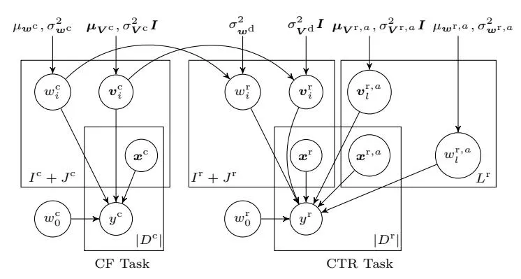
Fig. 1. Graphic model of transferred factorisation machines.

3.4 Dual-Task Bridge

To model the dependency between the two tasks, the weights of the user features and publisher features in CTR task are assumed to be generated from the counterparts in CF task (as a prior):

$\boldsymbol{w}^{\mathrm{r}} \sim \mathcal{N}(\boldsymbol{w}^{\mathrm{c}}, \sigma_{\boldsymbol{w}^{\mathrm{d}}}^{2} \boldsymbol{I}),$ (8)

where $\sigma_{\boldsymbol{w}^{d}}^{2}$ is the assumed variance of the Gaussian generation process between each pair of feature weights of CF and CTR tasks and the weight generation is assumed to be independent across features. Similarly, the latent vectors of CTR task are assumed to be generated from the counterparts of CF task:

$\boldsymbol{v}_{i}^{\mathrm{r}} \sim \mathcal{N}(\boldsymbol{v}_{i}^{\mathrm{c}}, \sigma_{\boldsymbol{V}^{\mathrm{d}}}^{2} \boldsymbol{I})$ (9)

where i is the index of a user or publisher feature; $\sigma_{V^{\text{d}}}^2$ is defined similarly.

The rational behind the above bridging model is that the users’ interest towards webpage content is relatively general and the displayed ad can be regarded as a special kind of webpage content. One can infer user interests from their browsing behaviours, while their interests on commercial ads can be regarded as a modification or derivative from the learned general interests.

The graphic representation for the proposed transferred factorisation machines is depicted in Figure 1. It illustrates the relationship among model parameters and observed data. The left part is for the CF task: $\boldsymbol{x}^{c}$ , $w_{0}^{c}$ , $\boldsymbol{w}^{c}$ and $\boldsymbol{V}^{c}$ work together to infer our CF task target $y^{c}$ , i.e., whether the user would visit a specific publisher or not. The right part illustrates the CTR task. Corresponding to CF task, $\boldsymbol{w}^{r}$ and $\boldsymbol{V}^{r}$ here represent user and publisher features’ weights and latent vectors, while $\boldsymbol{w}^{r,a}$ and $\boldsymbol{V}^{r,a}$ are separately depicted to represent ad features’ weights and latent vectors. All these factors work together to predict CTR task target $y^{r}$ , i.e., whether the user would click the ad or not. On top of that, for each (user or publisher) feature i of the CF task, its weight $w_{i}^{c}$ and latent vector $\boldsymbol{v}_{i}^{c}$ act as a prior of the counterparts $w_{i}^{r}$ and $\boldsymbol{v}_{i}^{r}$ in CTR task while learning the model.

Considering the datasets of the two tasks might be seriously unbalanced, we choose to focus on the averaged log-likelihood of generating each data instance

from the two tasks. In addition, we add a hyperparameter $\alpha$ for balancing the task relative importance. As such, the joint conditional likelihood in Eq. (1) is written as

$\left[\prod_{(\boldsymbol{x}^{c}, y^{c}) \in D^{c}} P(y^{c} | \boldsymbol{x}^{c}; \Theta)\right]^{\frac{\alpha}{|D^{c}|}} \cdot \left[\prod_{(\boldsymbol{x}^{r}, y^{r}) \in D^{r}} P(y^{r} | \boldsymbol{x}^{r}; \Theta)\right]^{\frac{1-\alpha}{|D^{r}|}}$ (10)

and its log form is