Joint Optimization Of Bid And Budget Allocation In Sponsored Search

ABSTRACT

This paper is concerned with the joint allocation of bid price and campaign budget in sponsored search. In this application, an advertiser can create a number of campaigns and set a budget for each of them. In a campaign, he/she can further create several ad groups with bid keywords and bid prices. Data analysis shows that many advertisers are dealing with a very large number of campaigns, bid keywords, and bid prices at the same time, which poses a great challenge to the optimality of their campaign management. As a result, the budgets of some campaigns might be too low to achieve the desired performance goals while those of some other campaigns might be wasted; the bid prices for some keywords may be too low to win competitive auctions while those of some other keywords may be unnecessarily high. In this paper, we propose a novel algorithm to automatically address this issue. In particular, we model the problem as a constrained optimization problem, which maximizes the expected advertiser revenue subject to the constraints of the total budget of the advertiser and the ranges of bid price change. By solving this optimization problem, we can obtain an optimal budget allocation plan as well as an optimal bid price setting. Our simulation results based on the sponsored search log of a commercial search engine have shown that by employing the proposed method, we can effectively improve the performances of the advertisers while at the same time we also see an increase in the revenue of the search engine. In addition, the results indicate that this method is robust to the second-order effects caused by the bid fluctuations from other advertisers.

Permission to make digital or hard copies of all or part of this work for personal or classroom use is granted without fee provided that copies are not made or distributed for profit or commercial advantage and that copies bear this notice and the full citation on the first page. To copy otherwise, to republish, to post on servers or to redistribute to lists, requires prior specific permission and/or a fee.

Categories and Subject Descriptors

H.3.5 [Information Systems]: Information Storage and Retrieval - Online Information Services; J.0 [Computer Applications]: General

Keywords

Budget allocation, Bid optimization, Sponsored search, Algorithms, Experimentation

1. INTRODUCTION

Sponsored search is a popular format of online advertising and is also the main revenue source for search engine companies. In sponsored search, a list of ads is displayed along with the organic search results in response to a given query. Sponsored search results are produced by a different mechanism from that of organic search, though they are displayed simultaneously and have similar appearance. Generally, the organic search results are mainly generated based on the relevance of each web page to the query, while the sponsored search results are generated based on an auction process [20, 2, 13].

An advertiser can create a number of campaigns under an account. In each campaign, he/she sets a campaign budget, builds several groups of ad copies (creatives), and bids on some keywords with their match types¹ for each ad group. Each keyword is an auction entry that is supposed to be triggered by some user queries. When a user submits a query, the search engine will first retrieve the most relevant ads as candidates according to a matching function between the bid keywords and the query. Then these candidate ads will participate in an auction, and some ads (e.g., with the largest expected revenue for the search engine) will win and be displayed on the search result page [13]. If an ad is clicked by the user, the corresponding advertiser will be charged by the search engine. Usually, the charged amount is determined by the generalized second price (GSP) [11] auction mechanism, which means that the advertiser’s cost of a click depends on the bid price of the next ad in the ranking list of the auction. When a campaign runs out of budget, it will not be

^∗This work was performed when the first and the second authors were interns at Microsoft Research Asia.

¹The match type might be exact match or broad match.

permitted to participate in any auctions until the budget is increased or the next budget period starts. For example, if the campaign budget is set at a monthly basis, the campaign will be re-involved in the auctions next month.

As can be seen above, besides creating ad groups and selecting bid keywords, an advertiser should also carefully consider two important problems as follows:

a) Bid Price Setting. Different keywords correspond to different opportunities (e.g., search volumes) and different degrees of competition. In many cases, the bids for some keywords are too low to win the auctions while the bids for some other keywords are unnecessarily high. Usually, the optimal bid price setting is very difficult for an individual advertiser to reach since he/she does not have the access to the related information (e.g., the bids of other advertisers) and his/her competitors are also adjusting their bid prices dynamically.

b) Campaign Budget Allocation. Similar to the case of keywords, different campaigns also have different opportunities and competition. As a result, under an account, some campaigns may run out of budget very quickly, some campaigns consume their budgets quite slowly, and the budgets for other campaigns may never be used at all. This will constrain the overall effectiveness for the advertiser to utilize his/her budget.

Both of the above issues are critical for advertisers, however, most advertisers have not been doing well in them according to our statistics (see Section 3). This is because many advertisers are managing hundreds of campaigns and tens of thousands of keywords, which makes it very difficult for them to manually tune the campaign budget allocation and keyword bid prices. There are some third-party tools to help the advertisers tune their bids; some advertisers even build tools themselves to manage the bids automatically. However, the market information they can get is still very limited, which restricts the effectiveness of the tools. In the research community, there have also been some attempts on preforming the task automatically (see Section 2). However, these works are still not sufficient to satisfy the practical requirements. For example, many works on keyword bid price optimization only consider the bid price when ranking the ads, but do not take relevance and position bias into consideration. For another example, although people have investigated keyword bid optimization, to the best of our knowledge, there is no work on campaign budget allocation yet in the literature.

In this paper, we propose a novel method to address the aforementioned issues. In particular, we propose jointly optimizing the campaign budget allocation and bid price setting. That is, for a given advertiser account with multiple campaigns and an account-level budget, we try to find the optimal allocation of the account-level budget into each campaign, and to set the optimal price^2,3 for each bid keyword in the campaign simultaneously. Here we focus on the joint

optimization instead of optimizing campaign budget allocation and keyword bid setting separately due to the following reason. Suppose for some campaign, there are many high-utility keywords (in other words, these keywords contain a lot of opportunities of advertising). In order to achieve significant performance regarding these keywords, one has to put a lot of money on them. However, if we cannot increase the budget for this campaign, we will miss a lot of these opportunities.

We formulate the problem as a constrained optimization, which takes the campaign budgets and the keyword bid prices as variables and finds their optimal values by maximizing the advertiser revenue, with the constraint of the account-level budget. To efficiently solve the optimization problem, we employ the sequential quadratic programming method. Simulation results on the sponsored search log from a commercial search engine show that the proposed technology can effectively help advertisers improve their campaign performance under several metrics like click number, cost per click, and advertiser revenue. At the same time, we can also help the search engine obtain increased revenue. In addition, the proposed method is robust to the second-order effects caused by the advertisers’ dynamical bid changes.

To sum up, the contributions of our work are listed as below. (i) We performed a comprehensive data study on the effectiveness of current campaign budget allocation and keyword bid price setting in sponsored search, and pointed out the importance and necessity of jointly optimizing them. (ii) We proposed a novel method for jointly optimizing bid and budget allocation. As far as we know, this is the first work on campaign budget allocation in the literature of sponsored search, and it is also the first work on consider keyword price setting and campaign budget allocation simultaneously.

As mentioned in the introduction, we focus on the joint optimization of campaign budget allocation and keyword bid price setting in this paper. That is, given an advertiser account with multiple campaigns and an account-level budget, we determine the optimal allocation of the account-level budget into each campaign, and set the optimal bid price for each bid keyword in the campaign. As far as we know, there is no work in the literature solving exactly the same problem. Instead, there is only some related work on keyword bid price optimization. We will briefly review such work in Section 2.1. Besides, there is some other work on budget allocation across different keywords [3], different search engines [8], or different online adverting markets [21], whose problem definitions are totally different with what we concern about in this paper.

2.1 Keyword Bid Price Setting

Chakrabarty et al [7] defined the weight and profit of each bid keyword, and proposed a knapsack based algorithm to find the optimal price setting that can maximize the advertiser revenue in sponsored search. The algorithm considered both single-slot and multi-slot auctions. Kitts et al [16] proposed a revenue optimization model based on the marketing factors that were related to ad slot positions, in order to solve the problem of keyword bid price setting. In [12, 17], a budget optimization problem was defined, in which the target is to find an optimal bid price setting to maximize the campaign performance under a given campaign budget.

^2Note that not all clicks are created equal. An advertiser will give different bids for different keywords, for they have different value per click (VPC). In this work, we estimate the VPC of a keyword based on the idea proposed in [4, 20] and use the VPC as the upper bound of the bid price.

^3Usually an advertiser observes the ad campaign performance and takes reactions to change the bid so as to approach the campaign goal. In this work, we find the optimal bid by maximizing the campaign goal directly, so the optimal bid is not a randomized value.

In particular, Feldman $et\ al\ [12]$ defined the cost and click functions considering the position of an ad and the average click-through rate (CTR) on the position, and then developed a landscape algorithm to solve the optimization problem in approximation. Muthukrishnan $et\ al\ [17]$ extended the above algorithm using a stochastic model, in which each keyword has a click distribution instead of an exactly known click number, in the context of single-slot auction.

In addition, the following works also discuss the problem of keyword bid price optimization, but in different scenarios from the above ones. Dar et al [10] studied how to improve the performance of broad match of bid keywords for a given query. They defined the weight and utility function of each bid keyword, and proposed a flow graph based algorithm to work out the optimal setting for keyword bid prices. Broder et al [6] pointed out that different matched queries for a bid keyword in broad match had different utilities according to their relevance to the bid keyword, and thus they should have different bid prices. They proposed a statistical approach to generate the corresponding bid prices. Borgs et al [5] studied the problem of keyword bid price setting given the budget on each keyword, and proposed an method to optimize the advertiser revenue across all keywords. More parts of the work are discussing the perturbation and convergence in their model.

3. DATA ANALYSIS ON SPONSORED SEARCH

In this section, we report our data analysis on sponsored search. We have used two kinds of data obtained from a mainstream search engine in our study: the auction log that records the detailed auction processes and the advertiser database that includes the bid keywords, bid prices, and the budget for each campaign. The data was collected in half a month, which contains over ten billion auctions and more than one hundred thousand advertiser accounts.

3.1 Campaign Budget

There can be several campaigns under the same advertiser account. In general, each campaign contains a set of ads (or ad groups) with the same campaign goal. Each campaign is assigned a budget, indicating the expected expense in a period of time (e.g., one month). In practice, due to the differences in the advertising settings and the market dynamics, it is quite common that some of the campaigns run out of budget while the other campaigns under the same account do not. We call this kind of accounts partially-running-out-of-budget accounts (or p-accounts for short). Here we give some statistics about the p-accounts in Table 1.

Table 1: Statistic of partially-running-out-budget accounts.

Number proportion	2.6%
Revenue proportion	31.6%
Potential revenue proportion	164.5%
Average campaign budget use ratio	45.1%
Total budget use ratio	11.5%
Average campaign number	15
Max campaign number	2,423
Average keyword number	10,735
Max keyword number	1,818,285

From Table 1 we have the following observations. (i) Although the number of the p-accounts is relatively small (2.6%), their contribution to the search engine revenue is

considerably large (31.6%). It is clear that the individual contribution of each p-account is much larger than that of other accounts. (ii) The potential revenue of the p-accounts⁴ is as much as 164.5% of the total revenue of sponsored search. This shows that improving p-accounts can result in a significant impact on the entire advertising system. (iii) The average campaign-level budget use ratio of the p-accounts is about 45.1%, and the total budget use ratio of the paccounts is 11.5%. The potential of further increasing the budget use ratio for the p-accounts is higher than for the other accounts. This is because the p-accounts have at least one campaign (but not all campaigns) running out of budget, thus we can further improve their budget use ratio by simply reallocating the residual budget to that campaign(s). However, for other accounts this strategy will not help. (iv) For a p-account, the average campaign number is 15 and the maximum campaign number is 2,423. These large numbers suggest that it is difficult to manually adjust the campaign budget.

3.2 Bid Price

Bid price setting is also a non-trivial task. For a p-account, the average number of bid keywords is 10,735 and the maximum is 1,818,285. It is clearly infeasible to manually set keyword bid prices for the p-accounts. Instead, automatic keyword bid price setting is desired. The tools from the third-party usually cannot have adequate market information to aid the bid tuning. For example, we may need to consider the following information. (i) First, according to the commonly-used auction mechanisms in commercial search engines, higher bid prices will increase the probability of winning more auctions and obtaining higher ranking positions. Figure 1 shows the percentage of ads that will get at least one position up if we increase their corresponding keyword bid prices to a certain degree. In particular, 57.36% ads will get position up if their keyword bid prices are increased by 10%, and 78.84% ads will get position up if their keyword bid prices are increased by 40%. (ii) Second, higher ranking positions usually mean more attention and clicks [15], according to Figure 2, which shows the relative CTR⁵ of the top ad slots in the commercial search engine. As a result, if an advertiser increases the bid price, the ad will have more opportunities to be clicked and the campaign goal of the advertiser will be better realized.

However, given the constraint of campaign budget, usually we cannot increase the bid prices for all the keywords. Instead, we have to balance between different keywords. Note that the utility of keywords are different from each other, and the return of lifting prices on some low-utility keywords might be very small. Therefore, we should consider the keyword utility when adjusting the keyword bid prices. For those keywords with low utility, the best choice may be to decrease their bid prices and instead put more money on the high utility keywords.

3.3 Joint Optimization

The data statistics reported in the previous section show that both campaign budget allocation and bid price setting are important to advertisers, but they are non-trivial to op-

$^4$ The potential revenue is calculated by summing up all the unused budgets of the p-accounts.

^5The relative CTR is normalized by dividing the CTR on each position by the CTR on the first position.

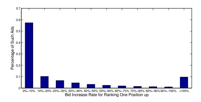
Figure 1: The proportion of ad volume ranking one position up with the increased bid price.

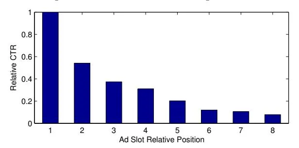
Figure 2: The relative CTR of each ad slot.

timize. If we want to jointly optimize them, the task may become even more difficult. However, we would like to point out that it is necessary to perform the joint optimization.

On one hand, if we only perform bid price optimization, each campaign will be optimized independently. For campaigns that have run out of budget, the help from bid price optimization will be limited because the potential capacity of these campaigns is constrained. For campaigns that have a lot of unused budget, bid price optimization can help achieve better performance, but it is hard to take full use of the budget due to the constraint of the value per click (VPC) of the bid keywords. On the other hand, if we only perform budget optimization, the unused budget will be reallocated to the campaigns that have already or tend to run out of budget, and thus their performance will be improved. However, the campaigns (no matter they run out of budget or not) will lose the opportunity to further improve their performance since their current bid price settings might not be optimal. Therefore, we had better consider both bid price optimization and campaign budget allocation simultaneously. In this way, the unused budget can be moved to the appropriate campaigns and can be effectively used on the best keyword candidates.

Note that in terms of optimizing the performances of advertisers, other efforts such as ad copy improvement, bid keyword selection, behavior and demography targeting, and landing page optimization are also important and effective. However, we will not discuss them as they are not in the scope of this paper.

4. JOINT OPTIMIZATION OF BID AND BUDGET ALLOCATION

In this section, we introduce the proposed method for joint optimization of bid price setting and campaign budget allocation. The key idea is to maximize the account-level ad-

vertiser revenue subject to the constraints of account-level budget. To better illustrate this idea, we first give some necessary notations including the definition of winning price interval, which serves as a basis of the following discussions. Then we adopt a probabilistic model to approximate the probability of winning a certain ad position given a bid price. After that, we define an optimization problem based on the probability model, and convert the problem to be a sequential quadratic programming problem. By solving the problem, we can get the optimal solution to campaign budget allocation and bid price setting.

4.1 Notations and Definitions

In the joint optimization of bid price setting and campaign budget allocation the input is an advertiser account $A = \{C_1, C_2, \ldots, C_m\}$ , where m is the number of campaigns under account A and $C_i (i = 1, 2, \ldots, m)$ is the i-th campaign. For simplicity, we will not distinguish ad group and ad in the following discussions. Accordingly, we can denote campaign $C_i$ as $C_i = \{g_i^{(0)}, D_i, K_i\}$ $(i = 1, \ldots, m)$ , where $g_i^{(0)}$ denotes the original periodical (e.g., monthly) budget set by the advertiser, $D_i$ denotes the set of ads, and $K_i$ denotes the set of bid keywords in campaign $C_i$ , respectively.

The ad set $D_i$ can be written as $D_i = \{d_{i,1}, d_{i,2}, \ldots, d_{i,l_i}\}$ , where $l_i$ is the number of ads in campaign $C_i$ and $d_{i,s}$ ( $s = 1, 2, \ldots, l_i$ ) denotes the s-th ad in the campaign. The bid keyword set $K_i$ can be written as $K_i = \{(k_{i,1}, b_{i,1}^{(0)}, v_{i,1}), (k_{i,2}, b_{i,2}^{(0)}, v_{i,2}), \ldots, (k_{i,n_i}, b_{i,n_i}^{(0)}, v_{i,n_i})\}$ where $n_i$ is the number of bid keywords⁸ in campaign $C_i$ , $k_{i,t}$ ( $t = 1, 2, \ldots, n_i$ ) denotes the t-th bid keyword, $b_{i,t}^{(0)}$ ( $t = 1, 2, \ldots, n_i$ ) denotes the original bid price for $k_{i,t}$ , and $v_{i,t}$ ( $t = 1, 2, \ldots, n_i$ ) denotes the VPC that $k_{i,t}$ brings. We approximately estimate the VPC based on the idea proposed in [4, 20], and regard it as the upper bound of $b_{i,t}^{(0)}$ [2, 11]. In addition, we denote the minimum reserve price as $\epsilon_b$ , which serves as the lower bound of the valid bids.

In sponsored search, the advertiser can associate several keywords to his/her ad. When a query is issued, an auction might be triggered. If one of the associated keywords of an ad matches the query by the corresponding match functions to the match types of the keywords, the ad (together with the matched keyword) will be involved in the auction. Therefore, the candidates in the auction is actually a tuple as $\omega_{i,s,t} = (d_{i,s}, (k_{i,t}, b_{i,t}^{(0)}, v_{i,t}))$ , where $s = 1, 2, \ldots, l_i$ and $t = 1, 2, \ldots, n_i$ . We call the tuple order item. For ease of reference, for an order item $\omega$ , we also use $(\cdot)_w$ to denote the attribute associate with it, such as its keyword $k_{\omega}$ , bid price $b_{\omega}$ , and VPC $v_{\omega}$ .

We use $\Phi$ to denote the maximum number of ad slots in each search result page of the sponsored search system. Suppose the ads are ranked in the auction according to their rank scores, then we have the following definitions.

DEFINITION 1 (WINNING SCORE). For an auction $\theta$ , its winning score at position $\rho_{\phi}$ (denoted by $\mu_{\phi,\theta}$ , $\phi = 1, 2, ..., \Phi$ )

^6In practice, the most relevant ad in an ad group will participate in the auction.

^7A keyword may have different match types and different bid prices accordingly. For simplicity, we regard them as different keywords.

^8The same keyword with different match types are regarded as different keywords in $K_i$ .

is the least rank score that can make an order item get the $\phi$ -th ad slot $\rho_{\phi}$ in the auction. Let $\mu_{0,\theta} = +\infty$ , then we have $\mu_{0,\theta} \geq \mu_{1,\theta} \geq \ldots \geq \mu_{\Phi,\theta}$ .

DEFINITION 2 (WINNING SCORE INTERVAL). For an auction $\theta$ , its winning score interval at position $\rho_{\phi}$ is $[\mu_{\phi,\theta},\mu_{\phi-1,\theta})$ ( $\phi=1,2,\ldots,\Phi$ ), which is the range of the rank score that can make an order item exactly get the $\phi$ -th ad slot $\rho_{\phi}$ in the auction.

Mainstream search engines use the product of the bid price and the quality score as the rank score in their auctions [13]. Suppose the quality score of an order item $\omega$ in an auction $\theta$ is $r_{\omega,\theta}$ , which can be calculated based on a group of features such as the query-ad similarity, semantic similarity, taxonomy, user query time, user query location and so on [14, 15, 19]. As indicated by the subscript, the quality score $r_{\omega,\theta}$ of an order item can be different in different auctions, due to some contextual information related to time, location, and user for the triggering query [14]. Usually such a quality score indicates the probability that an ad will be clicked after it is noticed by users. In this context, we have the following definitions of winning price and winning price interval.

DEFINITION 3 (WINNING PRICE). Given an order item $\omega$ in an auction $\theta$ with its quality score $r_{\omega,\theta}$ , its winning price at position $\rho_{\phi}$ (denoted by $\beta_{\omega,\phi,\theta}$ , $\phi=1,2,\ldots,\Phi$ ) is $\frac{\mu_{\phi,\theta}}{r_{\omega,\theta}}$ , which is the least bid price that can make $\omega$ get the $\phi$ -th ad slot $\rho_{\phi}$ in the auction. Let $\beta_{\omega,0,\theta}=+\infty$ , and we have $\beta_{\omega,0,\theta}\geq\beta_{\omega,1,\theta}\geq\ldots\geq\beta_{\omega,\Phi,\theta}$ .

DEFINITION 4 (WINNING PRICE INTERVAL). Given an order item $\omega$ in an auction $\theta$ with its quality score $r_{\omega,\theta}$ , its winning price interval at position $\rho_{\phi}$ is $[\beta_{\omega,\phi,\theta},\beta_{\omega,\phi-1,\theta}]$ ( $\phi=1,2,\ldots,\Phi$ ), which is the range of the bid price that can make $\omega$ exactly get the $\phi$ -th ad slot $\rho_{\phi}$ in the auction.

4.2 Probabilistic Model for Ad Ranking

In order to compute the expected advertiser revenue, we need to get the probability for an order item $\omega$ with bid price $b_{\omega}$ to be ranked at position $\rho_{\phi}$ in the auctions. More specifically, we define a probability distribution $P_{\omega}(b_{\omega})$ as,

$P_{\omega}(b_{\omega}) = (p_{\omega}(\rho_1|b_{\omega}), p_{\omega}(\rho_2|b_{\omega}), \dots, p_{\omega}(\rho_{\Phi}|b_{\omega}), p_{\omega}(\rho_{\Phi+1}|b_{\omega})),$

where $p_{\omega}(\rho_{\phi}|b_{\omega})$ ( $\phi=1,2,\ldots,\Phi$ ) denotes the probability for $\omega$ to be ranked in slot $\rho_{\phi}$ when its bid price is $b_{\omega}$ , and $p_{\omega}(\rho_{\Phi+1}|b_{\omega})$ denotes the probability for $\omega$ to lose the auction (i.e., to be ranked lower than $\rho_{\Phi}$ ). It is clear that,

$\sum_{\phi=1}^{\Phi+1} p_{\omega}(\rho_{\phi}|b_{\omega}) = 1.$

To get the above probability distribution, we apply the Bayes theorem to each element of it.

$p_{\omega}(\rho_{\phi}|b_{\omega}) = \frac{p_{\omega}(b_{\omega}|\rho_{\phi})p_{\omega}(\rho_{\phi})}{\sum_{j=1}^{\Phi+1} p_{\omega}(b_{\omega}|\rho_{j})p_{\omega}(\rho_{j})}$

Here $p_{\omega}(\rho_{\phi})$ is the probability of any ad being displayed at position $\rho_{\phi}$ in the auctions that $\omega$ participates in, which can be approximately obtained by simple counting in the historical auction log. $p_{\omega}(b_{\omega}|\rho_{\phi})$ is the probability of observing $b_{\omega}$ in the winning price interval at position $\rho_{\phi}$ in the auction

$\theta$ that $\omega$ participates in. A straightforward way is also to obtain this value by simple counting in the historical auction log. That is, for each auction $\theta$ of $\omega$ ( $\theta = 1, 2, \ldots, \Theta_{\omega}$ , where $\Theta_{\omega}$ denotes the number of auctions $\omega$ participates in.), we calculate the winning price interval $[\beta_{\omega,\phi,\theta},\beta_{\omega,\phi-1,\theta})$ for position $\rho_{\phi}$ from the auction log. If $b_{\omega} \in [\beta_{\omega,\phi,\theta},\beta_{\omega,\phi-1,\theta})$ , we say that there is an observation of price $b_{\omega}$ . However, the problem with this approach is that we need to go through the entire log for every possible value of $b_{\omega}$ , which will be too costly when we performing the optimization. Therefore we propose a new approach as described below that can be much more efficient without revisiting the entire auction logs during the optimization process.

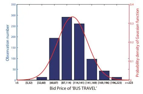
Figure 3: A case of Gaussian fitting for the bound of the winning price intervals.

For all auctions of $\omega$ , we can calculate their winning price intervals at position $\rho_{\phi}$ . As mentioned above, the lower bound and upper bound of the winning price interval are actually in fluctuation in different auctions. For simplicity, we use the following Gaussian distributions¹⁰ to model the fluctuation of the bounds.

$\begin{array}{rcl} q_{\omega}^{(L)}(x|\rho_{\phi}) & = & \frac{1}{\sqrt{2\pi\sigma_{\omega,\phi}^2}} e^{-(x-\bar{\beta}_{\omega,\phi})^2/2\sigma_{\omega,\phi}^2} \\ q_{\omega}^{(U)}(y|\rho_{\phi}) & = & \frac{1}{\sqrt{2\pi\sigma_{\omega,\phi-1}^2}} e^{-(y-\bar{\beta}_{\omega,\phi-1})^2/2\sigma_{\omega,\phi-1}^2} \end{array}$

Here x and y are the random variables for the lower bound and upper bound of the winning price interval of $\omega$ at position $\rho_{\phi}$ , and the superscripts L and U stand for lower bound and upper bound respectively. In addition, $\bar{\beta}_{\omega,\phi}$ and $\sigma_{\omega,\phi}$ are the mean and standard deviation for the lower bounds of the winning price intervals at position $\rho_{\phi}$ for all auctions of $\omega$ . That is,

$\begin{array}{rcl} \bar{\beta}_{\omega,\phi} & = & \frac{1}{\Theta_{\omega}} \sum_{\theta=1}^{\Theta_{\omega}} \beta_{\omega,\phi,\theta} \\ \sigma_{\omega,\phi}^2 & = & \frac{1}{\Theta_{\omega}} \sum_{\theta=1}^{\Theta_{\omega}} (\beta_{\omega,\phi,\theta} - \frac{1}{\Theta_{\omega}} \sum_{\theta=1}^{\Theta_{\omega}} \beta_{\omega,\phi,\theta})^2 \end{array}$

Similarly, $\bar{\beta}_{\omega,\phi-1}$ and $\sigma_{\omega,\phi-1}$ are the mean and standard deviation for the upper bounds of the winning price intervals at position $\rho_{\phi}$ for all auctions of $\omega$ .

^9Note that we compute this probability at the order item level but not for each individual auction, mainly because of the concern of data sparseness.

^10We have tested several possible distributions including Gaussian, Beta, and Gamma distributions, and found Gaussian is one of the best choices. Due to space limit, we will not show the parameter fitting for the distributions, but we can show an running example like Figure 3. As this is an approximation for the real data, we will ignore the negative values from the Gaussian distribution, just like what we usually do when we assume the heights of a group of people are sampled from a Gaussian distribution.

Thus $p_{\omega}(b_{\omega}|\rho_{\phi})$ can be computed as below.

$p_{\omega}(b_{\omega}|\rho_{\phi}) = p_{\omega}(x \leq b_{\omega} < y|\rho_{\phi})$

$= p_{\omega}(x \leq b_{\omega}|\rho_{\phi})p_{\omega}(b_{\omega} < y|\rho_{\phi})$

$= \int_{-\infty}^{b_{\omega}} q_{\omega}^{(L)}(x|\rho_{\phi})dx \int_{b_{\omega}}^{\infty} q_{\omega}^{(U)}(y|\rho_{\phi})dy$

$= \emptyset(\frac{b_{\omega} - \bar{\beta}_{\omega,\phi}}{\sigma_{\omega,\phi}})(1 - \emptyset(\frac{b_{\omega} - \bar{\beta}_{\omega,\phi-1}}{\sigma_{\omega,\phi-1}}))$

$(\phi = 2, \dots, \Phi)$

Here $\emptyset(\cdot)$ represents the cumulative distribution function of the standard normal distribution. In particular, for the first ad slot $\rho_1$ , the upper bound y is infinity. Hence $p_{\omega}(b_{\omega} < y|\rho_1) \equiv 1$ , and then,

$p_{\omega}(b_{\omega}|\rho_1) = p_{\omega}(x \le b_{\omega}|\rho_1) = \emptyset(\frac{b_{\omega} - \bar{\beta}_{\omega,1}}{\sigma_{\omega,1}}).$

Similarly, for $\rho_{\Phi+1}$ , the lower bound x is zero. Hence $p_{\omega}(x \leq b_{\omega}|\rho_{\Phi+1}) \equiv 1$ , and then,

$p_{\omega}(b_{\omega}|\rho_{\Phi+1}) = p_{\omega}(b_{\omega} < y|\rho_{\Phi+1}) = 1 - \emptyset(\frac{b_{\omega} - \bar{\beta}_{\omega,\Phi}}{\sigma_{\omega,\Phi}}).$

Figure 4 uses an example to explain the calculation of the probability $p_{\omega}(b_{\omega}|\rho_{\phi})$ . Suppose the bid of an observation is 28 (cents), then the probability $p_{\omega}(b_{\omega}|\rho_{\phi})$ equals to the product of the area of the left shadow (probability of lower bound < 28) and the area of the right shadow (probability of upper bound > 28).

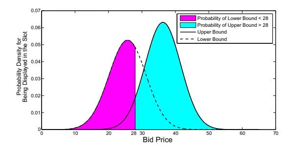
Figure 4: An example of the probability density distribution of the upper bound and lower bound of a winning price interval.

So far we have discussed our probabilistic model for ad ranking based on the ad auction log data. Compared with the conventional ranking models, the probabilistic model is smooth and easy to be directly optimized. Note that this model can be designed in other forms with different data formats in different scenarios.

4.3 Optimization Problem

Given the definition of the probabilistic model described in the previous subsection, we can define the expected advertiser revenue. To ease the illustration, we further introduce two notations as below. (i) $\tau_{\phi}$ - the position bias at slot $\rho_{\phi}$ . As discussed in Section 3.2, the relative CTR (shown in Figure 2) indicates the probability of ads in the position $\rho_{\phi}$ being noticed. Further considering the definition of quality score $r_{\omega,\theta}$ , the actual probability of an ad being clicked when ranked on the slot $\rho_{\phi}$ will be $\tau_{\phi}r_{\omega,\theta}$ [15]. (ii) $c_{\omega,\phi,\theta}$ - the cost for a click on $\omega$ in an auction $\theta$ where it is ranked on position $\rho_{\phi}$ . According to the GSP system, the cost can be calculated as $c_{\omega,\phi,\theta} = \frac{b_{\omega'}r_{\omega',\theta}}{r_{\omega,\theta}}$ , where $\omega'$ is the order item that is ranked one slot lower than $\omega$ in the auction $\theta$ , and $b_{\omega'}$ is its bid price.

The objective of the optimization problem is to maximize the total revenue of the advertiser account, which reflects the final profit the advertiser can make from the sponsored search. The constraints are the bounds of the bid prices and the campaign budget.

For all the campaigns in an advertiser account, the total expected click number can be written as

$\sum_{i=1}^{m} \sum_{\omega \in C_i} \sum_{\theta=1}^{\Theta_{\omega}} \sum_{\phi=1}^{\Phi} p_{\omega} (\rho_{\phi} | b_{\omega}) \tau_{\phi} r_{\omega, \theta}.$

where the factor $\sum_{\phi=1}^{\Phi} p_{\omega}(\rho_{\phi}|b_{\omega})\tau_{\phi}r_{\omega,\theta}$ is the probability of click on $\omega$ in one auction when the bid price is $b_{\omega}$ .

Considering the cost of click and the VPC of each bid keyword, we can get the expected advertiser revenue as follows,

$\sum_{i=1}^{m} \sum_{\omega \in C_i} \sum_{\theta=1}^{\Theta_{\omega}} \sum_{\phi=1}^{\Phi} p_{\omega}(\rho_{\phi}|b_{\omega}) \tau_{\phi} r_{\omega,\theta} (v_{\omega} - c_{\omega,\phi,\theta}).$

Given the above objective function, we can formulate the joint optimization as below, where $g_i$ $(i=1,2,\ldots,m)$ and $b_{\omega}$ denote the variables of campaign budgets and keyword bid prices respectively. The minimum campaign budget is $\epsilon_g$ , for the advertiser might not like to entirely close a campaign by letting $g_i = 0$ .

$\max_{g_{i},b_{\omega}} \sum_{i=1}^{m} \sum_{\omega \in C_{i}} \sum_{\theta=1}^{\Theta_{\omega}} \sum_{\phi=1}^{\Phi} p_{\omega}(\rho_{\phi}|b_{\omega}) \tau_{\phi} r_{\omega,\theta}(v_{\omega} - c_{\omega,\phi,\theta})$

$s.t. \qquad \sum_{i}^{m} g_{i} = \sum_{i}^{m} g_{i}^{(0)}$

$0 \leq \sum_{\omega \in C_{i}} \sum_{\theta=1}^{\Theta_{\omega}} \sum_{\phi=1}^{\Phi} p_{\omega}(\rho_{\phi}|b_{\omega}) \tau_{\phi} r_{\omega,\theta} c_{\omega,\phi,\theta} \leq g_{i}$

$(i = 1, 2, \dots, m)$

$\epsilon_{g} \leq g_{i} \quad (i = 1, 2, \dots, m)$

$\epsilon_{b} \leq b_{\omega} \leq v_{\omega} \quad (\omega \in C_{i}, i = 1, 2, \dots, m)$

4.4 Efficient Solution

The above optimization problem is a typical constrained optimization problem. It can be approximately solved by means of sequential quadratic programming (SQP) [9] in an efficient manner.

Suppose $\xi_1 = \{b_\omega\}$ ( $\omega \in C_i$ , i = 1, 2, …, m) denotes the vector of bid prices for all the order items in an advertiser account, and $\xi_2 = \{g_i\}$ (i = 1, 2, …, m) denotes the vector of campaign budgets. Then $\xi = (\xi_1^T, \xi_2^T)^T$ is the vector of all variables. We can rewrite the optimization problem as the following form.