Modeling Indirect Effects Of Paid Search Advertising

Many online shoppers initially acquired through paid search advertising later return to the same website directly. These so-called “direct type-in” visits can be an important indirect effect of paid search. Because visitors come to sites via different keywords and can vary in their propensity to make return visits, traffic at the keyword level is likely to be heterogeneous with respect to how much direct type-in visitation is generated.

Estimating this indirect effect, especially at the keyword level, is difficult. First, standard paid search data are aggregated across consumers. Second, there are typically far more keywords than available observations. Third, data across keywords may be highly correlated. To address these issues, the authors propose a hierarchical Bayesian elastic net model that allows the textual attributes of keywords to be incorporated.

The authors apply the model to a keyword-level data set from a major commercial website in the automotive industry. The results show a significant indirect effect of paid search that clearly differs across keywords. The estimated indirect effect is large enough that it could recover a substantial part of the cost of the paid search advertising. Results from textual attribute analysis suggest that branded and broader search terms are associated with higher levels of subsequent direct type-in visitation.

Key words: Internet; paid search; Bayesian methods; elastic net

1. Introduction

In paid search advertising, marketers select specific keywords and create text ads to appear in the sponsored results returned by search engines such as Google or Yahoo!. When a user clicks on the text ad and is taken to the website, the resulting visit can be attributed directly to paid search. Existing research has focused on modeling traffic and sales generated by paid search in this direct fashion (e.g., Ghose and Yang 2009, Goldfarb and Tucker 2011, Rutz et al. 2010). In these models, the effectiveness of paid search is evaluated by attributing any ensuing direct revenues and pay-per-click costs to keywords or categories of keywords. These approaches assume implicitly that if a consumer does not purchase in the session following the click-through, the money

¹ A notable exception is a dynamic model developed by Yao and Mela (2011). By leveraging bidding history information in a unique data set from a specialized search engine in the software space, the authors are able to infer present and future advertiser value arising from both direct and indirect sources.

spent on that click is “lost”; i.e., it has not generated any revenue. This line of research has not yet addressed the subsequent revenues that may be generated by consumers returning to the site. Revenues (e.g., sales, subscriptions, referrals, display ad impressions) generated by site visitors who arrive by means not directly traced to paid search are typically considered to be separate. Visitors, however, could decide not to purchase at the first (paid search originated) session but return to the site later either to view more content or perhaps to complete a transaction. Indeed, after initially coming to a site as a result of a paid search, consumers could return again and again, creating an ongoing monetization opportunity. The problem of quantifying these indirect effects of paid search is similar to the one described by Simester et al. (2006) in the mail-order catalog industry. They point out that a naïve approach to measuring the effectiveness of mail-order catalogs omits the advertising value of the catalogs and that targeting decisions based on models without indirect effects produce suboptimal results. In the case of paid search advertising, ignoring indirect effects can positively bias the attribution of sales to other sources of site traffic and downwardly bias keyword-level conversion rates.

Consumers can access a website by typing the company’s URL into their browser or using a previously visited URL (stored either in the browser’s history or previously saved “bookmarks”). Because these visits occur without a referral from another source, they fall into the class of traffic known as nonreferral, and we label them direct type-in visits.² Referral visits can be due to paid search (the consumer accesses the site via the link provided in the text ad at the search engine), organic search (the consumer clicks on a non-paid, organic link at the search engine), or other Internet links, such as clicking on a banner advertisement. In this paper, we focus on referrals from a search engine (both organic and paid) and their impact on future nonreferral visits (the so-called direct type-in). Specifically, we are interested in how past paid search visits affect the current number of direct type-in visits to a site.

Shoppers formulate their search queries in different ways depending on their experience, shopping objectives, readiness to buy, and other factors. Indeed, managers at the collaborating firm that provided our data—an automotive website—told us that when they switched off some keywords, a drop in direct type-in visitors occurred “a couple of days later,” whereas switching off others did not affect future direct type-in traffic. We posit that self-selection into the use of different keywords may reflect the propensity of a paid search visitor to return to the site later via direct type-in. This proposition is consistent with previous research in paid search (e.g., Ghose and Yang 2009, Goldfarb and Tucker 2011, Rutz et al. 2010, Yao and Mela 2011) that showed heterogeneity of direct effects across keywords. We seek to contribute to this stream of research by expanding this notion of keyword-level heterogeneity into the domain of indirect effects. For example, imagine two consumers wanting to buy a DVD player. One of them searches for “weekly specials Best Buy DVD player” and the other for “Sony DVD player deal.” An ad for http://www.bestbuy.com is displayed after both searches, and both consumers click on the ad. From Best Buy’s perspective, it seems more likely that the consumer who searched for Best Buy’s weekly specials will revisit the site. This leads to the notion that keywords may be proxies for different types of consumers and/or search stages. Thus, they may be more or less effective for the advertiser based on potential differences in their indirect effects on future traffic, and one might posit that each keyword has its own specific indirect effect. From the firm’s perspective, the indirect effect is important to quantify to effectively manage paid search advertising.

There are several challenges in doing this. First, there is typically no readily available consumer-level data that firms can use to accurately identify a “return” visit. Hence, attribution of future direct typein traffic to keyword-level paid search traffic needs to be done based on aggregate data. Second, the number of keywords managed by the firm is often much larger than the number of observations, e.g., days, available. Finally, paid search traffic generated by subsets of keywords is frequently highly correlated. To handle these problems, we introduce a new method to the marketing literature: a flexible regularization and variable selection approach called the elastic net (Zou and Hastie 2005). We adopt a Bayesian version of the elastic net (Li and Lin 2010, Kyung et al. 2010) that allows us to estimate keyword-level indirect effects across thousands of keywords even with a small number of observations. We also extend the literature on Bayesian elastic nets by incorporating a hierarchy on the model parameters that inform variable selection. This allows us to leverage information the keyword provides by introducing semantic keyword characteristics. To extract these semantic characteristics from keywords, we introduce an original structured text-classification procedure that is based on managerial knowledge of the business domain and design elements of the website. The proposed procedure is extendable to other data sets and is easy to implement.

We test our model on data from an e-commerce website in the automotive industry. From our perspective, the indirect effects should be especially pronounced in categories such as big-ticket consumer durable goods, where the consumer search process is long (e.g., Hempel 1969, Newman and Staelin 1972). Given the nature of the product and evidence for a prolonged search process (e.g., Klein 1998, Ratchford et al. 2003), we believe that this category is well suited to study indirect effects in paid search. For example, Ratchford et al. (2003) find that consumers, on average, spend between 15 and 18 hours searching before purchasing a new car.

Our intended contribution is both methodological and substantive. Methodologically, given its robust performance in handling very challenging data sets (i.e., many predictors, few observations, correlation), we believe that the (Bayesian) elastic net will find many useful applications among marketing practitioners and academics. To the best of our knowledge, we are the first to introduce this model to the marketing field. Moreover, we offer an important extension to this model by allowing the variable selection

² Note that the term “direct type-in” should not be confused with the direct effect of paid search.

parameters to depend on a set of predictor-specific information in a hierarchy. Substantively, we expand the paid search literature by introducing another dimension of keyword performance—propensity to generate return traffic. We find significant heterogeneity in indirect effects across keywords and demonstrate that propensity to return is, in part, revealed through the textual attributes of the keywords used. Our empirical findings offer new insights from text analysis and should help firms to more accurately select and evaluate keywords.

The rest of this paper is structured as follows. First, we give a brief introduction to paid search data and discuss the motivation for our modeling approach. We then present our model, data set, and results. Next, we discuss the implications of our findings for paid search management. We finish with a conclusion, the limitations of our approach, and a discussion of future research in search engine marketing.

2. Modeling Approach and Specification

We propose to examine indirect effects of paid search by modeling the effect of previous paid search visits on current direct type-in visits. Our goal is to do this based on the type of readily available, aggregate data provided to advertisers by search engines, along with easily tracked visit logs from company servers.

2.1. Aggregate vs. Tracking Data

Ideally, firms would have consumer-level data at the keyword level tracked over time. Although the “ideal” scenario is attractive, our view is that it is effectively infeasible. There are two places where these data can be potentially collected—firms’ websites or consumers’ computers. All other intermediate sources (such as search engines and third-party referral sites) cannot provide a complete picture of the interaction between consumers and firms. For example, Google may be able to track all paid and organic visits to firms’ websites originated from its engine, but it will not have much information about direct visits or traffic generated through referrals. Needless to say, because of consumer privacy concerns, search engines are highly unlikely to share consumer-level data with advertisers (e.g., Steel and Vascellaro 2010). Alternatively, tracking on the consumers’ end could be implemented by either recruiting a panel or using data from a syndicated supplier who maintains a panel. Unfortunately, the size of such a panel needed to ensure adequate data on the keywords used by a given firm would be impractical—especially for less popular keywords in the so-called “long tail.” Crosssession consumer tracking on firms’ websites is also problematic for several reasons—practical, technical, and corporate policy. First, firms may require each entering visitor to provide log-in identification information that can help with tracking across multiple visits. Although this approach is indeed used for existing customers of some sites—often subscriptiontype services (e.g., most of the features of Netflix or Facebook require users to be logged in)—it is unlikely to be effective with new customers. Because new customer acquisition is one of the primary goals of paid search advertising, asking for registration at an early stage is likely to turn many first-time visitors away. Second, although tracking is typically implemented by use of persistent cookies,³ this approach has become less reliable in recent years. Current releases of major Internet browsers (e.g., Internet Explorer, Mozilla Firefox, Google Chrome) support a feature that automatically deletes cookies at the end of each session. In addition, many antivirus and antiadware programs—now in use on more than 75% of Internet-enabled devices (PC Pitstop TechTalk 2010) do the same. Although there seems to be no consensus on the percentage of consumers who delete cookies regularly, reported numbers range up to 40% (Quinton 2005, McGann 2005). A cookie-based tracking approach would misclassify any repeat visitor as a new visitor if the cookie was deleted, biasing any estimate that is based on the ensuing faulty repeat versus new visitor split. Finally, as a corporate policy, many companies in the public sector (39% of state and 56% of federal government websites) and some companies in the private sector (approximately 10%) simply prohibit tracking across sessions (West and Lu 2009).

In the absence of tracking data, aggregate data are available that capture how visitors have reached the site. Visitors to any given website are either referral or nonreferral visitors. A nonreferral visit occurs if a consumer accesses the website by typing in the company’s URL, uses a URL saved in the browser’s history, or uses a previously saved (“bookmarked”) URL. We call these visits direct type-in. A referral visit is one that comes from another online source. For example, consumers can use a search engine to find the site and access it by clicking on an organic or a paid search result.⁴ In this paper, we focus on visitors referred by search engines and call these organic and paid search visits. We note that the proposed model can be extended to accommodate other referral traffic such as banner ads or links provided by listing services such as Yellow Pages.

³ IP address matching is another alterative, but as Internet service providers commonly use dynamic addressing and corporate networks “hide” the machine IP address from the outside world, it is mostly infeasible.

⁴ Companies can also try to “funnel” consumers to their site by using online advertising. A company can place a banner ad on the Internet, and consumers can access the company’s site by clicking on that banner ad.

2.2. Method Motivation

From a methodological perspective, the objective of our study is to demonstrate how a modified version of the Bayesian elastic net (BEN; e.g., Li and Lin 2010, Kyung et al. 2010) can be used in marketing applications where (1) the number of predictor variables significantly exceeds the number of available observations, (2) predictors are strongly correlated, and (3) model structure (but not just a forecasting performance) is of focal interest to the researcher or practitioner. Zou and Hastie (2005, p. 302), who coined the term “elastic net,” describe their method using the analogy of “a stretchable fishing net that retains all the big fish.” Indeed, the method is meant to retain “important” variables (big fish) in the model while shrinking all predictors toward zero (therefore letting small fish escape). We offer an extension to the Bayesian elastic net model proposed by Kyung et al. (2010) by incorporating available predictor-specific information into the model in a hierarchical fashion. Before we present the details of the proposed model, we offer a brief motivation for our selected statistical approach.

Normally, when the number of observations significantly exceeds the number of predictors, estimation/evaluation of the effects of individual predictors is straightforward. However, when the number of predictors is substantially larger than the number of observations, estimation of individual parameters becomes problematic. The model becomes saturated when the number of predictors reaches the number of observations. Using terminology proposed by Naik et al. (2008), the paid search data we use fall into a category of so-called VAST (Variables × Alternatives × Subjects × Time) matrix arrays where the V dimension is very large compared with all other dimensions. The problem of having a large number of predictors coupled with a relatively low number of observations is referred to as the “large p, small n” problem (West 2003). Naik et al. (2008) review approaches to the “large p, small n” problem and identify the following three broad classes of methods—regularization, inverse regression, and factor analysis. The following conditions, found in our empirical application, make these approaches unsatisfactory: (1) the focus of the analysis is on identifying all relevant predictors that help to explain the dependent variable, rather than just on forecasting; (2) more than n predictors should be allowed to be selected; and (3) subsets of predictors may be strongly correlated. The first condition rules out methods that reduce dimensionality by combining predictors in a manner that does not allow recovery of predictor-level effects. For example, methods such as partial inverse regression (Li et al. 2007), principal components (e.g., Stock and Watson 2006), or factor regressions (e.g., Bai and Ng 2002) make such inference difficult. Some regularization techniques, such as Ridge regression (e.g., Hoerl and Kennard 1970), do not allow subset selection but instead produce a solution in which all of the predictors are included in the model. The second condition eliminates techniques that become “saturated” when the number of predictors reaches the number of observations. For this reason models such as LASSO regression (e.g., Tibshirani 1996, Genkin et al. 2007) are not applicable in our context. Although LASSO allows exploring the entire space of models, the “best” model cannot have more than n predictors selected. Finally, methods that address dimensionality reduction perform poorly when high correlations exist among subsets of predictors. The multicollinearity problem is particularly important in high dimensions when the presence of related variables is more likely (Daye and Jeng 2009). For example, regularization through a standard latent class approach (i.e., across predictors) or with LASSO may fail to pick more than one predictor from a group of highly correlated variables (Zou and Hastie 2005, Srivastava and Chen 2010).

Another class of methods that can potentially address the above conditions is based on a two-group discrete mixture prior with one mass concentrated at zero and another somewhere else—also known as the so-called “spike-and-slab” prior (e.g., Mitchell and Beauchamp 1988). This class of models is generally estimated by associating each predictor with a latent indicator that determines group assignment (e.g., George and McCulloch 1993, 1997; Brown et al. 2002). Bayesian methods are commonly used to explore the space of possible models and to determine the best model as the highest frequency model (stochastic search variable selection, or SSVS). Although this class of methods has been shown to perform well in a “typical” (n > p5 setting (e.g., Gilbride et al. 2006), the application to a “large p, small n” context is not without limitations, and computational issues arise for large p (Griffin and Brown 2007).⁵

The Bayesian elastic net belongs to the class of regularization approaches and is designed to handle the above-mentioned three conditions. Like Ridge regression, it allows more than n predictors to be selected in the “best” model. Like LASSO, it offers a sparse solution (not all available predictors are selected) and

⁵ As p becomes large, it becomes hard to identify high-frequency models—the key outcome of the SSVS approach (Barbieri and Berger 2004). Consequently, for high-dimensional problems the posterior mean or BMA (Bayesian model averaging) estimator is typically used. Because a BMA estimator naturally contains many small coefficient values, it does not offer a sparse solution (Ishwaran and Rao 2010), which is of interest in our case. Though BMA improves on variable selection in terms of prediction, its drawback is that it does not lead to a reduced set of variables (George 2000). allows for grouping across predictors; strongly correlated predictors are added to or excluded from the model together. In the modeling situation described by the above conditions and faced by firms in the paid search domain, the Bayesian elastic net offers a very good match as a state-of-the-art approach to the “large p, small n” problem.

2.3. Bayesian Elastic Net

We specify as our dependent variable the number of direct type-in visitors to the website at a given time t (DirV). In our data this activity is tracked at the daily level. We investigate the effect, if any, of prior paid search visits (PsV) on the number of direct type-in visitors. Our model allows for keyword-level effects, which we see as an empirical question. We also account for seasonal effects, i.e., using daily and monthly dummies, and for variations in overall website traffic patterns by using lagged organic visitors (OrgV) as a control. Finally, potential feedback effects are incorporated by including lagged direct type-in visitors. We use an exponentially smoothed lag structure (ESmo), allowing us to estimate only one parameter per keyword. Our model is given by

$DirV_{t} = \alpha + \sum_{i=1}^{6} \beta_{i}^{\text{day}} I_{t}^{\text{day}} + \sum_{i=1}^{4} \beta_{i}^{\text{month}} I_{t}^{\text{month}} + \lambda DirV_{t}^{ESmo} + \delta OrgV_{t}^{ESmo} + \sum_{k=1}^{K} \phi_{k} PsV_{t}^{ESmo,k} + \varepsilon_{t},$

$(1)$

$DirV_{t}^{ESmo} = \sum_{l=1}^{L_{DirV}} w_{l}^{DirV} DirV_{t-l}, \quad \sum_{l=1}^{L_{DirV}} w_{l}^{DirV} = 1,$ $w^{DirV} = (w_{1}^{DirV} \cdots w_{L_{DirV}}^{DirV})',$ $OrgV_{t}^{ESmo} = \sum_{l=1}^{L_{OrgV}} w_{l}^{OrgV} OrgV_{t-l}, \quad \sum_{l=1}^{L_{OrgV}} w_{l}^{OrgV} = 1,$ $w^{OrgV} = (w_{1}^{OrgV} \cdots w_{L_{OrgV}}^{OrgV})',$ $PsV_{t}^{ESmo,k} = \sum_{l=1}^{L_{PsV}} w_{l}^{PsV} PsV_{t-l}^{k}, \quad \sum_{l=1}^{L_{PsV}} w_{l}^{PsV} = 1,$ $w^{PsV} = (w_{1}^{PsV} \cdots w_{L_{DSV}}^{PsV})',$

⁶ A consistent finding of paid search research (e.g., Ghose and Yang 2009) is heterogeneity in response across keywords. One possible reason could be consumer “self-selection” into keywords—consumers reveal information on preferences through the use of keywords.

⁸ Alternatively, we could specific the lag structure explicitly. However, this would require us to estimate multiple (i.e., the number of lags) parameters per keyword—a steep increase for cases in which the firm bids on thousands of keywords. To be consistent, we also use exponential smoothing on DirV and OrgV.

$w_{l}^{\dots} = \frac{\exp(-l \times \zeta)}{\sum_{k=1}^{L_{\dots}} \exp(-k \times \zeta)},$

where $DirV_t$ is the number of direct type-in visitors at time t, $\{I_t^{\rm day}, I_t^{\rm month}\}$ is a set of daily and monthly indicator variables, $OrgV_t$ is the number of organic visitors at time t, $PsV_t^k$ is the number of paid search visitors from keyword k at time t, K is the number of keywords the firm is using, $\varepsilon_t \sim N(0, \sigma^2)$ and $\alpha$ , $\beta = (\beta_1^{\rm day} \cdots \beta_6^{\rm day} \beta_1^{\rm month} \cdots \beta_4^{\rm month})'$ , $\lambda$ , $\delta$ , $\phi = (\phi_1 \cdots \phi_K)'$ , and $w^{DirV}$ , $w^{OrgV}$ , $w^{PsV}$ , $L^{DirV}$ , $L^{Org}$ , $L^{PsV}$ , $\zeta$ , and $\sigma$ are parameters (vectors) to be estimated.

A challenge in estimating Equation (1) is that most firms bid on hundreds or even thousands of keywords. Based on the available daily data provided by search engines, firms would need to run search campaigns for multiple years before one would be able to estimate the model given in Equation (1). For example, our focal company bid on over 15,000 keywords. One way to address this problem is to estimate the model specified in Equation (1) for each individual keyword at a time (controlling for all other variables). A problem with this approach is that the daily traffic generated by different keywords is correlated. The bias from omitting the effects of other keywords in Equation (1) is likely to produce inflated estimates for the role of any given individual keyword in generating returning direct type-in visitors.

To address this challenge, we propose a Bayesian elastic net (Kyung et al. 2010) that discriminates among keywords based on their effectiveness using a Laplace-Gaussian prior to address the data deficiency. The prior ensures that “weaker” predictors get shrunk toward zero faster than “stronger” predictors (see also Park and Casella 2008). A BEN allows us to estimate keyword-level parameters even when the number of keywords is significantly larger than the number of observations ( $n \ll p$ ). The Laplace– Gaussian prior encourages a grouping effect, where strongly correlated predictors are selected or dropped out of the model together. Finally, it allows for the best model to include more than n predictors. Our modeling approach also has been designed to directly address concerns expressed by practitioners. We have been told that “when we turn off sets of keywords, we see a drop in the number of visitors that come to the site directly. That drop has a time delay of a couple of days.” The goal of our model is to identify which keywords drive this effect, allowing us to measure the additional indirect value these particular keywords have above and beyond generating site visits via paid search click-through.

Along with data on traffic, firms have detailed keyword lists. In general, keywords can be decomposed into certain common semantic characteristics, e.g., a keyword is related to car financing. We propose a

^<sup>7 Organic visits can have a similar effect as paid visits. A consumer accesses the site through an organic link and might be coming back as a direct visitor going forward.

novel text mining approach to extract semantic characteristics from keywords (for details, see the section on empirical application), allowing us to leverage semantics to shed light on why some keywords are effective and others are not. To this end, we propose a hierarchical model that can incorporate predictorspecific information such as semantics. Note that an elastic net shrinks all predictors to zero—a typical feature of regularization approaches. Thus, contrary to the way in which hierarchies on parameters have been implemented in the marketing literature, we cannot impose a hierarchical mean on the keywordspecific parameter ^k in the standard fashion. In a BEN, parameters determine the amount of shrinkage toward zero and thus have a significant influence on the parameter estimate. Our hierarchy is based on these parameters and we define the BEN prior as follows:

$\phi \propto \exp\left[-\frac{1}{\sqrt{\sigma^2}} \sum_{k=1}^K \kappa_{1k} |\phi_k| - \frac{1}{2\sigma^2} \sum_{k=1}^K \kappa_{2k} \phi_k^2\right].$ (2)

We define the hierarchy on the keyword-specific parameters 1^k and 2^k as follows:

$\kappa_{1k} \sim \text{gamma}(c_{1k}, d) \quad \text{and} \quad \kappa_{2k} \sim \text{gamma}(c_{2k}, d), \quad (3)$

where c1^k and c2^k are parameters to be estimated for all keywords.⁹ We use a log-normal model to represent the effect of the semantic keyword characteristics on c1^k and c2^k :

\log(c_i) \sim N\left(U\theta_i, v_i^2\right), \quad i = 1, 2, \tag{4}

where U is a 4K × S5 matrix of semantic keyword characteristics, S is the number of semantic keyword characteristics, cⁱ is a 4K × 15 parameter vector containing cik, and ⁱ 4S × 15 and ⁱ 41 × 15 are parameters (vectors) to be estimated. (For details, see Web Appendix A in the electronic companion to this paper, available as part of the online version that can be found at http://mktsci.pubs.informs.org/.) Our integrated Bayesian approach addresses the dimensionality issue with the Laplace–Gaussian prior and provides a parsimonious solution to an otherwise intractable problem. Our approach provides two key benefits. First, it enables us to estimate the indirect effect on a keyword level. Second, our hierarchical BEN allows us to investigate whether differences in keyword effectiveness can be traced back to semantic keyword characteristics.

We have also addressed two common modeling concerns, endogeneity and serial correlation. In our modeling situation, endogeneity may arise from two potential sources: managerial reaction (feedback mechanism) to changes in direct traffic and omitted variable bias. We probed extensively for endogeneity, and none of the tests we conducted indicate that endogeneity is of concern (for details, please see Web Appendix B in the electronic companion). To address concerns with regard to serial correlation, we include an AR415 error process in our model (e.g., Koop 2003) implemented in a fully Bayesian framework (for details, please see Web Appendix A in the electronic companion).

2.4. Model Comparisons

We compare our proposed model against two benchmarks. First, we model direct type-in visits without including paid search as an explanatory variable (NO KEYWORDS). This is implemented by estimating Equation (1) without PsV. Second, we model direct type-in visits assuming all keywords have the same (homogeneous) effect, i.e., setting ^k = 1∀k (ALL KEYWORDS). Our proposed model follows the specification described in Equations (1)–(4) above and is labeled BEN. Moving from NO KEYWORDS to ALL KEYWORDS enables us to assess the presence and magnitude of the indirect effect but at an aggregate (across all keywords) level. Moving from ALL KEYWORDS to BEN enables us to determine the keyword-level effect on direct type-in visits and the value of modeling the indirect effect on a keyword level.

3. Data

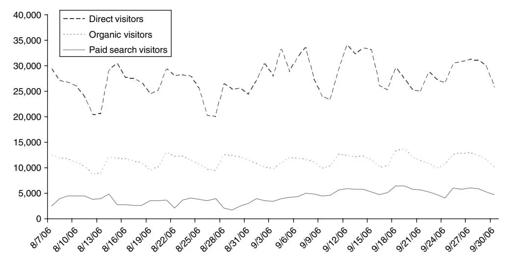
3.1. Data Set Description

Our empirical application is based on a data set from a commercial website in the automotive industry.¹⁰ Almost all commercially available cars and light trucks are offered, prices are fixed (no haggling policy), and consumers can either order their new cars online or obtain referrals to a dealership. The company also brokers after-market services such as financing and roadside assistance. The data set spans 117 days, from May to September 2006. The company tracks how visitors come to its website: typing in the URL or using a bookmark (direct type-in visits per day, DirV), clicking on an organic search result (organic visits per day, OrgV), or clicking on a paid search result (paid search visits per day, PsV). The majority of the visits to the site (see Figure 1) are direct type-in visits (63%, daily average of 30,669 visits). Organic visits account for 27% of the traffic (daily average of 13,248 visits), and paid search visits account for 10% (daily average of 4,791 visits). Note that the company focused its advertising

⁹ Note that a gamma has a location (c > 0) and a scale (d) parameter. We set the scale parameter d = 1 for identification.

¹⁰ The company wishes to stay anonymous.

strategy on paid search alone—it did not use banner ads nor links on other websites nor advertise offline. The data set also includes information on daily paid search traffic obtained through Google AdWords: the number of daily impressions and clicks, and the average cost per click. Because of the wide range of products and services the company offers, the campaign consisted of 15,749 keywords. Paid search led, on average, to 230,392 impressions and 4,791 clicks (or visits) per day (see Table 1). The average cost per click (CPC) is $0.33, resulting in an average daily spending of $1,568 on paid search for Google. The average click-through rate (CTR) is 2.1%. Over the 117-day period, 560,558 paid search visits (i.e., clicks) to the site generated a cost of $183,559. Revenue stemmed from selling cars and services as well as from advertisements on the site. Nearly all car makers advertise on the site and are charged based on the number of page views. Thus, even if a consumer does not buy from the company, he still generates advertising revenue by browsing the site.

As noted previously, a key challenge in estimating individual keyword effects is that the number of keywords is much larger than the number of observations. In our case, we need to estimate the effects of 15,749 keywords from 117 data points (see Table 2). From a practical perspective, it seems unlikely that all keywords would have a strong effect on return visits. For example, keywords that do not lead to clicks are unlikely candidates for generating direct visitors after the search. A paid search ad consists

Table 1 Paid Search Campaign Summary Statistics

Paid search	Impressions	Clicks	Cost ($)	CPC ($)	CTR (%)
Total Daily average	26,955,850 230,392	560,558 4,791	183,559 1,568	0.33	2.1

of two lines of text and competes for attention with many other paid ads as well as organic results. Thus, we feel that it is very unlikely that a searcher who did not click on a paid search ad memorizes the URL displayed in the ad and types it in at a later point to visit the site. In our 117-day sample period, almost half of the keywords (7,312) did not generate any clicks at all, and we exclude these from further consideration. We also note that our data exhibit the long-tail phenomenon generally found in paid search campaigns. In our case, 96% of the cost is spent on the 38% (3,186) of keywords with 10 clicks or more over the observation period. From a managerial perspective, focusing on these keywords seems valid. The remaining keywords (those not in the top 3,186) have very few observations over the period of the data. Indeed, one might expect any algorithm to struggle with those keywords. We tested our model using simulated data and find that very sparse predictors are not recovered with any reasonable accuracy. We therefore propose that excluding all keywords with fewer than 10 clicks¹¹ might be the best approach to the problem. Thus, we focus our investigation on the top 3,186 keywords. 12

^<sup>11 We also tested other cutoff points in the same range and find that our semantic inference is not affected by the cutoff point.

$^{^{12}}$ Dropping a subset of predictors (keywords) could bias our semantic analysis of keyword effectiveness (for an example, see Zanutto and Bradlow 2006). Given that we focus on evaluating the effects of semantic characteristics on the keyword’s propensity to generate return visits (but not paid search traffic), the subsampling used in our case is not conditioned on the dependent variable $(\phi_i)$ , but rather it is based on an associated summary measure (i.e., paid search visits). If $\phi_i$ and paid search visits are independent, then there is no need for correction, because the dropped $\phi_i$ can be viewed as missing at random. The analysis of our empirical results reveals that there is a trivial correlation between $\phi_i$ and paid search visits. However, if this correlation is found to be nontrivial,

Table 2 Summary Statistics for All Keywords vs. Focal Keywords

	Impressions	Clicks	Cost		CPC ($) CTR (%)
All keywords (15,749)
Total Daily average	26,955,850 560,558 $183,559 230,392	4,791	$1,568	0.33	2.1
Focal keywords (3,186)
Total	24,177,614 521,016 $171,420			0.33	2.2
(Percentage of all keywords)	(86.0)	(92.9)	(95.9)
Daily average	206,646	4,453	$1,465

3.2. Extracting Semantic Information

One of the questions we address in this study is whether useful semantic information can be extracted from keywords to understand differences in indirect effects. Current academic research on this topic is in its early stages, and very few papers on paid search consider semantic properties of key phrases (e.g., Ghose and Yang 2009, Yang and Ghose 2010, Rutz et al. 2010). In these papers, only a few attributes characterizing a keyword are handpicked in an ad hoc manner—e.g., retailer name, brand name, or geographic location. A consistent finding is that these keyword characteristics have statistical power in predicting click-through rates and purchases. Based on these findings, we posit that a semantic analysis could also prove effective in understanding differences across keywords when it comes to predicting return visitation propensity. However, we believe that existing ad hoc procedures of dummy coding can be improved by introducing a more structured approach. In this paper, we propose a novel two-stage approach to extract semantic keyword attributes. In the first step, we identify potentially relevant attributes allowing us to “decompose” keywords. In the second step, each keyword is coded using the identified attributes. In the extreme, each word or combination of words can be treated as a unique attribute. The downside of this approach is the dimensionality of the estimation problem—the attribute space formed by unique words can easily become unmanageable. Dimensionality reduction can be achieved by creating a set of attributes where each attribute is associated with multiple words. For example, words such as “Ford,” “Toyota,” and “Honda” can be described by the attribute “Make.” Hence, the keyword “Toyota Corolla lease” contains the attributes “Make,” “Model,” and “Financial.” If the

we suggest that the proposed model can be expanded to address the subsampling problem. Specifically, we may assess the correlation between ⁱ and the corresponding paid search visits based on the retained keywords only, and we adjust for selection bias when estimating the effects of semantic attributes , assuming that this correlation holds true for low-volume keywords as well (e.g., in the spirit of a Tobit model).

set of attributes (e.g., “Make”) and associated words (e.g., “Ford,” “Toyota,” “Honda”) are known, keyword coding can easily be automated. The key challenges, however, lie in attribute definition. First, we need to determine what attributes should be used to characterize the underlying keywords; e.g., in the automotive domain, “Make,” “Model,” “Year,” and “Financial” might be among potential candidates. Second, we need to determine which words are associated with each attribute; e.g., we need to know that “Leasing” and “Payments” should be associated with the attribute “Financial.” One way to approach this problem is to use cluster analysis techniques designed for qualitative data (e.g., Griffin and Hauser 1993). The basic idea behind this class of methods is to consider the entire set of words that need to be assigned into an unspecified number of clusters. Clustering and classification are done simultaneously by human coders. The downside of this approach is that implementation becomes quite costly when the number of words to be classified becomes large.

The approach proposed in this paper also requires human input with regard to the cluster (attribute) definition; however, overall, it is less labor intensive than existing approaches. Specifically, we start by collecting unstructured data that describe the business domain of the collaborating firm. Two sources of information are considered in this respect: interactions with firm’s management and content of the firm’s website. We then manually analyze the collected data to identify the set of attributes capturing different aspects of the firm’s business, which might be of interest to the target market and, hence, might be searched for online. Finally, we use these attributes to characterize (code) available keywords. In contrast to the cluster analysis techniques discussed above, our proposed procedure can be seen as a top-down approach to classification, where we define clusters first and then assign keywords to them. From a practical standpoint, the downside of this approach is that it is possible to miss some semantic dimensions that might differentiate keywords. On the other hand, our approach may help to discover dimensions of the business environment not yet covered by the set of keywords used by the firm. As another benefit, once the set of attributes has been defined, the remaining classification task is fully automated.¹³

We now outline the key steps taken to extract semantic attributes from keywords.

Step 1. Based on a set of interviews, questionnaires, and/or other communications with the firm’s management, identify the key areas of business in which

¹³ For the expanded version of this procedure and detailed examples, please refer to Web Appendix C in the electronic companion.

the firm is offering services to consumers.¹⁴ For example, “Car sales,” “Vehicle pricing,” “Auto insurance,” and “Financial service” were among the identified areas.

Step 2. For each of the identified business areas, define a set of words that would (preferably unambiguously) describe the corresponding area. For example, “Financial services” is associated with “Leasing,” “Financing,” “Credit,” and “Loan.”

Step 3. Extract cognitive synonyms (synsets) and hypernyms for each word defined in Step 2 using the application program interface of the public domain tool WordNet 2.1¹⁵ (Miller 1995). For example, for “Financing,” the term “Funding” is a synonym and “Finance” is a hypernym.

Step 4. Perform stemming (word reduction to its base form; see Lovins 1968) for both the list of words generated in Step 3 and all the words found in keywords used by the firm in a paid search. For example, for “Funding,” the base form is “Fund.”

Step 5. For each keyword used by the firm, find the match in the list of synonyms or hypernyms generated in Step 3. If a match is found, code the corresponding keyword on the matched attribute.

Step 6. Review the list of classified keywords; if needed, expand the list of synonyms and repeat from Step 4.

Step 7. For the remaining nonclassified keywords (if any), introduce additional descriptive categories (e.g., code all conjunctions as category “Grammar”).

In application to our data set, the proposed approach yields a list of 30 characteristics, of which 29 were coded as indicator variables in the empirical model. Note that more than one attribute can be associated with each keyword because most keywords in our empirical data set contain two words or more and/or because some of the individual words are classified into more than one category. Specifically, only 2% of keywords were associated with a single indicator, whereas 23%, 54%, 19%, and 3% of keywords were described by 2, 3, 4, and 5 or more indicators, respectively. Although the proposed procedure is not fully automated, it significantly reduces the effort needed to classify keywords based on semantic characteristics. Another promising direction for using keyword information is to leverage developments in text mining and natural language processing (e.g., from applications based on user-generated content). Several recent studies have argued that usergenerated media, i.e., “the language of the consumer,” may serve as an indispensable resource to understand consumers’ preferences, interests, and perceptions (Archak et al. 2007, Bradlow 2010, Feldman et al. 2010). Although the application of text mining to paid search has not yet appeared in marketing, we believe it has significant potential.

4. Estimation Results

4.1. Model Selection

We use a predictive approach to assess model fit and to determine model selection. Specifically, we base our analysis on the posterior predictive distribution using so-called posterior predictive checks (PPCs).¹⁶ Calculating PPCs requires generating predicted (or replicated) data sets based on the proposed model and the parameter estimates. Comparing these predictions to the observed data is generally termed a posterior predictive check (e.g., Gelman et al. 1996, Luo et al. 2008, Braun and Bonfrer 2010, Gilbride and Lenk 2010). PPCs offer certain advantages over standard fit statistics. First, a wide range of diagnostics can be defined based on the distribution of predictions under a model. Second, posterior predictive simulation explicitly accounts for the parametric uncertainty that is usually ignored by alternative approaches. Using PPCs we can not only evaluate whether a proposed model provides the best fit compared with other models but we can also investigate whether the proposed model adequately represents the data. However, model checking by means of PPCs is openended, and gold standards have yet to be established (Gilbride and Lenk 2010). We use PPCs to investigate model fit in-sample as well as model predictive power out-of-sample.

As discussed above, in a posterior predictive check we compare predicted data sets with the actual data set at hand. These comparisons are based on so-called discrepancy statistics T . A large number of potential discrepancy statistics is available, and the researcher is faced with an inherent trade-off. Some statistics, e.g., root mean square discrepancy (RMSD) as used by Luo et al. (2008), utilize the whole data to describe fit, whereas others, e.g., minimum and maximum as suggested Gelman et al. (1996), allow investigation of model fit on certain dimensions of

¹⁴ A similar procedure was followed to identify key functional areas of the website design. Although many of the functional areas overlap with the business areas identified by the firm’s management, there was a significant number of unique functional attributes. For example, photo gallery, newsletter, and specific make and model information all are functional attributes.

¹⁵ WordNet® is a large lexical database of English, developed under the direction of George A. Miller. Nouns, verbs, adjectives, and adverbs are grouped into sets of cognitive synonyms (synsets), each expressing a distinct concept. Synsets are interlinked by means of conceptual-semantic and lexical relations. The resulting network of meaningfully related words and concepts can be navigated with the browser (source: http://wordnet.princeton.edu/).

¹⁶ We thank an anonymous reviewer for this suggestion.

Table 3 Posterior Predictive Checks

		(a) In-sample
Model	RMSD	MAD	MAPD
NO KEYWORDS	3,291	2,606	0.1194
ALL KEYWORDS BEN	1,838 804	1,451 621	0.0721 0.0205
		(b) Out-of-sample
Model	RMSD	MAD	MAPD
NO KEYWORDS ALL KEYWORDS BEN	3,386 1,875 1,087	2,738 1,485 583	0.1479 0.0877 0.0263

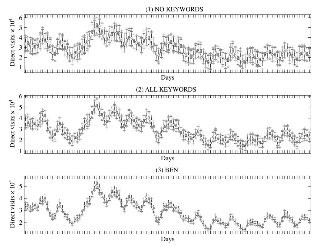
interest, e.g., the tails. We acknowledge this tradeoff and investigate how the model fits the data on a global level as well as on specific dimensions of interest to the researcher.¹⁷ To test for fit on a global level, we use statistics such as RMSD, mean absolute discrepancy (MAD), and mean absolute percentage discrepancy (MAPD). In our case, a regression model with a specific type of shrinkage structure, the data are relatively basic compared with many marketing applications, e.g., no individual-level data as in Gilbride and Lenk (2010). As such, we focus our investigation on specific dimensions of fit using different descriptives: fit in the tails by investigating minimum, maximum, and the 25%, 50%, and 75% quantiles. In addition, we also investigate fit of the model with regard to an important moment, the variance. We do this because with models of our type, overfitting in-sample and poor fit out-of-sample are concerns. Finally, we provide box-and-whiskers plots following Braun and Bonfrer (2010) to illuminate how well the different models describe the data based on the predicted data sets.

4.1.1. In-Sample. Following Gelman et al. (1996), we simulate sets of predicted DirVpred at each sweep of the sampler and calculate the proposed discrepancy statistics to investigate how close the predicted values (DirVpred5 resemble observed values (DirV). Based on the set of discrepancy statistics that capture the whole data (RMSD, MAD, and MAPD), we find that the proposed BEN model outperforms the NO KEYWORDS and the ALL KEYWORDS models (see Table 3, panel a). Inspecting the figures with respect to the posterior predictive densities, we see that the models replicate the data well (see Figures 2(a) and 2(b)). The BEN, in general, provides a better fit in-sample as shown by the smaller variances for the posterior predictive densities. This is also supported by the p-values reported (see Figures 2(a) and 2(b)). Moreover, close inspection of the box-and-whiskers plots (see Figure 3) indicates that the BEN is fitting the data better. We expect a model like ours to outperform a simpler model in-sample. The more critical question is whether a model with a large number of parameters—which can lead to overfitting in-sample—will also outperform a much simpler model in terms of out-of-sample.

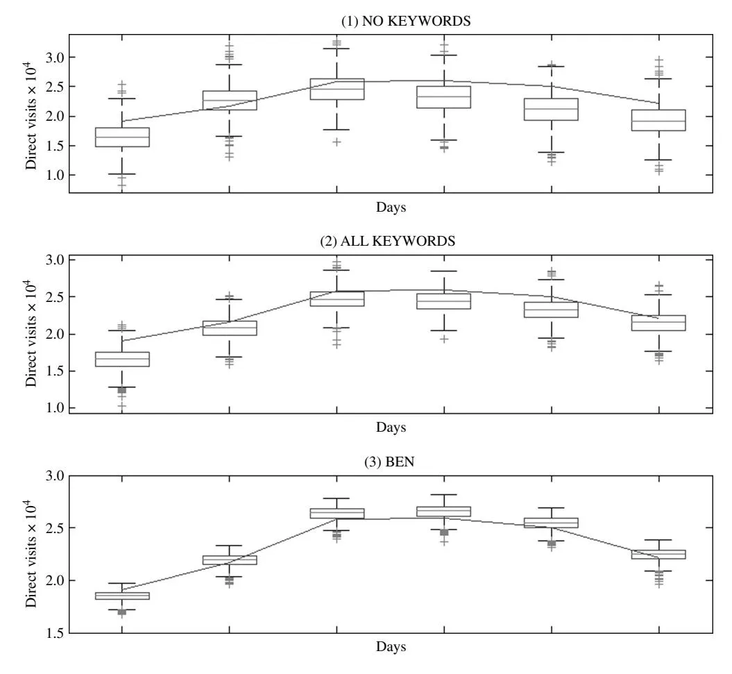
4.1.2. Out-of-Sample. We hold out the last week of the data and reestimate our models using the remaining 110 data points. Based on our estimates at each step of the sampler, we predict a set of DirVpred_^F for the holdout sample. We use the same set of discrepancy statistics as in sample. We find that our proposed BEN outperforms the NO KEYWORDS and the ALL KEYWORDS models (see Table 3, panel b). This alleviates the concern that in-sample overfitting might be driving model selection. Comparing the densities, we find that the BEN replicates the data well. Compared with the ALL KEYWORDS and the NO KEY-WORDS models, the BEN provides a better forecast (as shown by the significantly smaller variance of all the posterior predictive densities; see Figures 4(a) and 4(b)). This is again supported by the p-values (see Figures 4(a) and 4(b)). As was true in-sample, the box-and-whiskers plots show the BEN to be better at capturing the data points in the holdout sample (see Figure 5)—i.e., it is closer to the true value and provides a forecast with a smaller variance.

4.2. Coefficient Estimates

In Table 4, we present the estimated model coefficients for our proposed approach (BEN) along with those for the two benchmark models (NO KEY-WORDS and ALL KEYWORDS). We will focus our discussion on the estimates for the BEN model.¹⁸ The model effectively captures the seasonality present in online activity and the auto industry. First, online activity is much higher during the week and falls off during the weekend (Pauwels and Dans 2001). The highest direct type-in traffic occurs on Mondays (included in the intercept) with increasingly negative estimates for the daily dummy variables as the week progresses. Second, accounting for monthly effects reveals the typical summer seasonality in the auto industry. Turning to the effects of previous direct type-in, organic, and paid search visits on future direct type-in visits, we calculate both short- and long-run effects.¹⁹ We find that the mean immediate (i.e., next period) effect of DirV is 0.53 and the mean long-run effect is 1.15. The effect for an organic visit (OrgV) is similar: the mean immediate effect is 0.57

¹⁷ We thank the editor for this suggestion.

¹⁸ In our empirical investigation we set 2^p = ² for all p. We also investigated a full model and found the results to be very similar. ¹⁹ We do this at each sweep of the sampler based on effect_LR = effect_SR/41 − 5 and report the mean of the effects.

Figure 2(a) PPCs—In-Sample

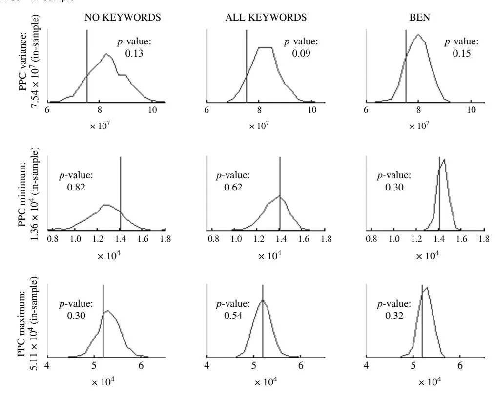
Figure 2(b) PPCs by Quantile—In-Sample

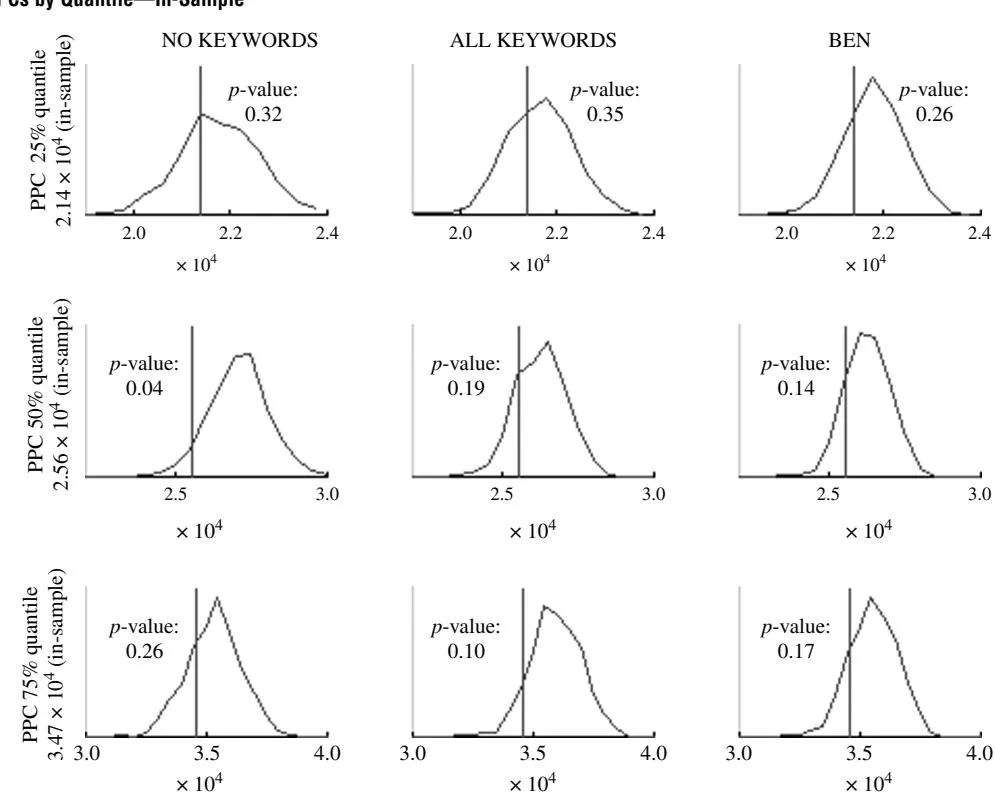
Figure 3 Box-and-Whiskers Plot—In-Sample

and the mean long-run effect is 1.23. The posterior mean of the exponential smoothing parameter is 2.97 ( = 0048), indicating that any lags beyond t − 2 have virtually no effect.²⁰ We find evidence for serially correlated errors; the posterior mean of based on an AR415 process is 0.24 ( = 0009).

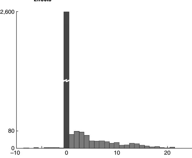
We now discuss whether keywords differ with respect to the effects that they have on future direct type-in visits. Based on our BEN model, we find that effects differ significantly across keywords. First, of the 3,186 keywords, 599 have a significant indirect effect; i.e., the 95% highest posterior density (HPD) coverage interval does not contain zero. Figure 6 presents a histogram of the estimated posterior mean keyword-level parameters. The large spike at zero represents the 2,587 keywords that have no significant indirect effect. We also analyzed some of the properties of the 599 keywords identified as having significant effects. For example, these keywords represent 66% of the paid search clicks (341,360) but only 54% (13,586,685) of the impressions (see Table 5). Note that the click-through rate on the significant keywords is higher: 2.5% versus 1.7%. This potentially indicates that the keywords that better match user needs also attract visitors with a higher propensity to return to the site. Of the 599 significant keywords, 57 generate more than 1,000 clicks over the observation period, whereas 132 have between 999 and 100 clicks and 410 have fewer than 100 clicks. For the insignificant keywords, only 15 keywords have more than 1,000 clicks and the large majority (2,306) have fewer than 100 clicks (see Table 6).

In our setting, the majority of consumers should have a relatively lengthy search process because of the nature of the automotive category (e.g., Klein 1998, Ratchford et al. 2003). We believe that our results using daily search data provide, in the best case, a good estimate of the indirect effect and in the worst case (i.e., many intraday and fewer across-days searchers), a lower bound for the indirect effect. To be sure, more return visits could be occurring within a day, which is hard to identify given a daily aggregated data set. The fact that we find a significant indirect effect across days highlights the importance of this phenomenon. Whereas some advertisers are now able to examine intraday data, we note that it is likely to bring other modeling challenges along with it, e.g., sparse data in the overnight hours.

In sum, the extent to which paid search brings consumers to the site also explains variation in subsequent direct type-in visits. This is an important empirical finding because it indicates that investments in paid search advertising may pay dividends to firms above and beyond their immediate effects. Second, we find that not all paid search visits are “the

²⁰ For example, based on using up to three lags, the weight of time period t − 1 is 94.9%, t − 2 is 4.8%, and t − 3 is 0.3%.

Figure 4(a) PPCs—Out-of-Sample

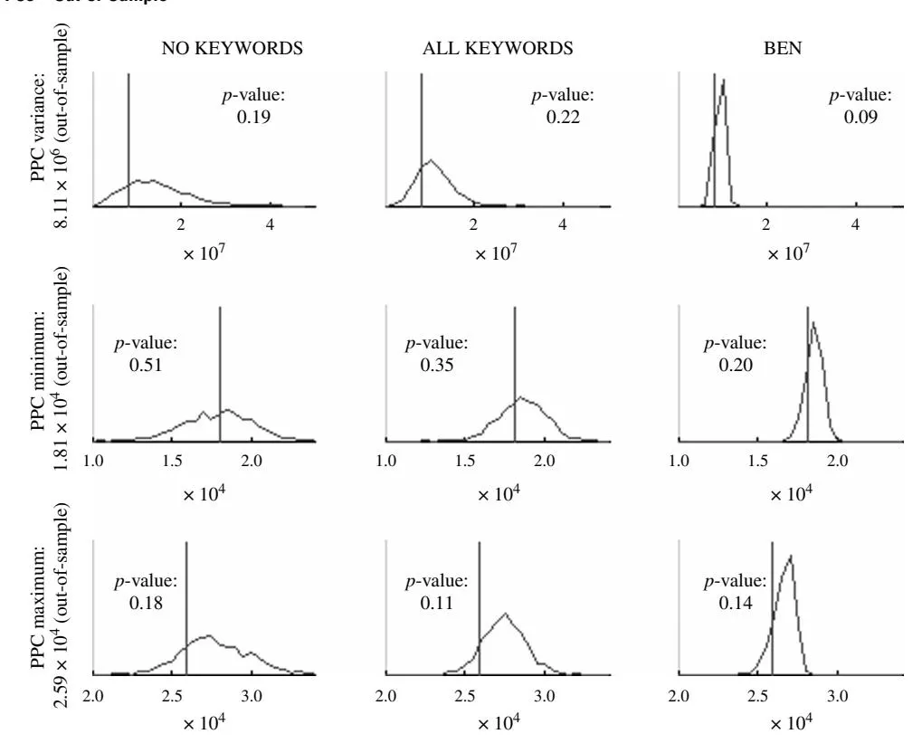
Figure 4(b) PPCs by Quantile—Out-of-Sample

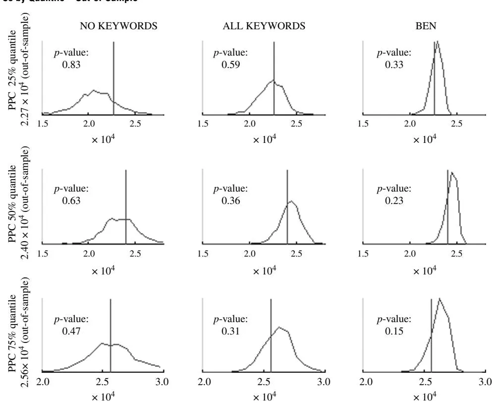
Figure 5 Box-and-Whiskers Plot—Out-of-Sample

same.” In particular, keyword-level data are useful in investigating how an advertiser can drive “good” consumers to a website. In our case, a subset of 599 keywords can be associated with bringing consumers back to the site via direct type-in at significantly higher rates than other keywords.

5. Managerial Implications

5.1. General Findings

We find two classes of keywords with respect to generating future repeat visits: 2,587 keywords are not effective, whereas 599 keywords can be linked to fluctuations in direct type-in traffic. We now ask how to value this indirect effect. Advertising (by car makers) on the site accounts for a significant part of company revenue. Every viewed page that displays banner ads generates incremental advertising revenue, because banner ads are billed on an exposure basis. Using our results, we estimate the ad revenue generated by the additional direct type-in visits attributable to paid search and then contrast it with the actual costs of the paid search campaign. Our evaluation is conservative in that some repeat visitors may subsequently go on to purchase from the company or be referred to a dealer, both of which generate substantial income. Because of data limitations, our analysis does not incorporate these additional benefits from repeat visitation. On average, a direct type-in visitor views 2.7 pages with advertising.²¹ Based on average advertising revenue of $31.59 per 1,000 page views, the value of a direct type-in visitor in terms of advertising revenue is roughly $0.08. Our model estimates imply that, in the long run, significant keywords generate, on average, about 3.3 return visitors per click (or $0.26 in advertising revenue). The average CPC for significant keywords is $0.22. Thus, our analysis indicates that an advertising profit of about $0.04 per click is generated by the significant keywords. Indeed, the total value of the estimated additional advertising revenue is $90,385.²² This recoups approximately 49%

²¹ The average number of page views for a direct visitor is 10.9. Note that not all pages have revenue-generating advertising on them.

²² Calculated as P class revenue × LR_effect × no0 of clicks.

		Coefficient estimatesa
Covariates		NO KEYWORDS	ALL KEYWORDS	BEN
Intercept		4,863.9 (1,269.4, 8,503.2)	4,375.5 (2,219.1, 6,524.9)	4,380.3 (2,806.5, 6,034.4)
Tuesday	day ’ 1	−2,781.8 (−4,566.3, −896.9)	−1,951.4 (−2,997.1, −945.4)	−2,110.9 (−2,911.9, −1,245.1)
Wednesday	day ’ 2	−5,587.7 (−7,342.7, −3,777.0)	−3,681.4 (−4,789.9, −2,568.1)	−4,054.4 (−4,884.5, −3,183.3)
Thursday	day ’ 3	−6,937.0 (−8,708.6, −5,245.9)	−5,289.1 (−6,354.7, −4,269.7)	−5,400.6 (−6,228.2, −4,585.4)
Friday	day ’ 4	−7,112.7 (−8,773.1, −5,496.4)	−6,076.3 (−7,140.5, −5,114.4)	−6,244.5 (−7,020.9, −5,433.2)
Saturday	day ’ 5	−8,191.1 (−9,939.7, −6,482.6)	−7,387.8 (−8,444.8, −6,387.3)	−7,720.7 (−8,502.0, −6,958.4)
Sunday	day ’ 6	−5,963.7 (−7,643.0, −4,343.3)	−5,404.5 (−6,322.2, −4,419.0)	−5,644.0 (−6,368.0, −4,928.0)
June	month ’ 1	5,442.9 (3,633.2, 7,011.5)	7,445.8 (6,360.5, 8,523.8)	5,431.0 (4,651.5, 6,241.5)
July	month ’ 2	6,937.8 (4,127.2, 9,493.1)	7,021.1 (5,473.8, 8,567.3)	7,267.0 (6,008.6, 8,570.3)
August	month ’ 3	1,171.6 (−731.8, 3,056.9)	1,491.7 (432.4, 2,643.6)	523.2 (−343.3, 1,436.4)
September	month ’ 4	1,928.2 (−35.0, 3,798.2)	−675.4 (−1,847.9, 618.8)	1,173.9 (264.9, 2,048.7)
Direct	‹	0.691 (0.595, 0.783)	0.434 (0.368, 0.499)	0.529 (0.488, 0.572)
Organic	”	0.531 (0.349, 0.721)	0.474 (0.373, 0.576)	0.566 (0.485, 0.651)
All keywords	”	—	1.865 (1.628, 2.107)	—

^aWe report posterior means as well as 95% HPD intervals.

of the total spending on paid search of $183,559 (see Table 1).

When simply inspecting the top significant keywords, we see that terms with the firm’s brand name

Figure 6 Histogram of the Posterior Means of Individual Keyword Effects

and very general terms such as “Buy car,” “Cars,” and “Car sales” have the highest number of clicks. The top insignificant keywords are very narrow searches such as “Toyota Avalon specs” and “Used Pontiac Vibe,” as well as terms that relate to selling a car such as “Used car selling.”²³ Although we cannot show a complete list of the keywords here, we note that significant terms often appear broader than insignificant terms. Empirically, we have observed in this data set and in other paid search data sets that broader keywords, e.g., “Cars online,” are more expensive (we believe mostly because of heightened competition). In our data this remains true even when holding position constant. Whereas the broader keywords are more expensive, it is not clear which type of keyword (based on CPC) would be more prone to attract visitors who are more likely to return via direct type-in. Indeed, when computed for the significant 599 keywords, the correlation between keyword effectiveness

²³ Note that the company had only recently started to sell and offer used cars and was not yet an established venue for selling used cars.

Table 5 Significant vs. Insignificant Keywords—Summary Statistics

Paid search	Impressions	Clicks	Cost ($)	CPC ($)	CTR (%)
Significant effect	13,586,685	341,360	110,926	0.32	2.5
Insignificant effect	10,590,929	179,656	60,493	0.34	1.7

Table 6 Significant vs. Insignificant Keywords—Click Perspective

Paid search	Clicks >1,000	999–500	499–100	<100
Significant effect	57	23	109	410
Insignificant effect	15	27	239	2,306

in generating return visits and CPC (CTR) is −0.04 (−0.15). This suggests that campaign statistics, e.g., CPC or CTR, may not be good proxies for indirect effects. We investigate in the next section whether semantic keyword characteristics help to better understand observed differences in indirect effects across keywords.

We end this section by contrasting the implications of the BEN model with the ALL KEYWORDS benchmark model. If one were to rely on the aggregate effect estimated from the ALL KEYWORDS model, this could significantly bias the indirect value of paid search. In this model the mean long-run effect of a paid search visit is 3.9 direct type-in visits, implying $0.32 in revenue. The additional advertising revenue would be $650,017—a severe overestimation of the additional revenue of $90,385 indicated by the superior BEN model.

5.2. Investigating Semantic Keyword Characteristics

We investigate whether semantic keyword characteristics can be used to understand keyword effectiveness in driving direct type-in traffic. In our BEN model, semantic keyword characteristics enter in a hierarchical fashion via the mean c¹ of the shrinkage parameters based on a log-normal model (i.e., we model log4c¹ 5). In our setup, a higher mean will lead to a higher , which in turn will introduce more shrinkage of the parameter toward zero and increase the probability that the corresponding keyword has no significant indirect effect. We find that semantic keyword characteristics explain variation in the mean of ¹ ; the mean R 2 for this regression is 0.23.²⁴ We group the semantic keyword characteristics into three classes for ease of exposition: one with negative effects, one with positive effects, and one with no significant effects (see Table 7 for results). Beginning with the semantic characteristics that have a negative effect (less shrinkage), we find that keywords

Table 7 Results for Semantic Keyword Characteristics

Semantic characteristic	Estimatea	Coverage intervalb	Change in shrinkagec (%)
Intercept	0048	(0.46, 0.51)	N/A
Auto	−0018	(−0.20, −0.16)	−5001
Buying	−0003	(−0.04, −0.02)	−707
Car	−0017	(−0.20, −0.15)	−4607
Comparison	−0002	(−0.04, −0.01)	−601
Image	−0027	(−0.30, −0.23)	−7206
Grammar	−0010	(−0.11, −0.09)	−2704
Information	−0010	(−0.12, −0.09)	−2802
Make	−0002	(−0.02, −0.01)	−402
Model	−0005	(−0.06, −0.04)	−1302
Sale	−0004	(−0.05, −0.03)	−1106
Search	−0026	(−0.29, −0.23)	−6907
Company	−0039	(−0.49, −0.28)	−10703
Web	−0007	(−0.09, −0.05)	−1801
Truck	0003	(0.01, 0.05)	904
Category	0007	(0.05, 0.09)	1906
Channel	0002	(0.01, 0.03)	503
Condition	0033	(0.28, 0.37)	8906
Inventory	0008	(0.05, 0.10)	2105
Feature	0006	(0.04, 0.08)	1602
Mileage	0028	(0.25, 0.32)	7702
Price	0014	(0.12, 0.16)	3809
Financial	0001	(−0.01, 0.02)	—
Selling	0002	(−0.01, 0.04)	—
Vehicle	−0002	(−0.04, 0.01)	—
Year	−0010	(−0.14, 0.05)	—
New	−0003	(−0.07, 0.03)	—
Used	−0004	(−0.09, 0.03)	—
Word Count	0011	(−0.10, 0.29)	—
NewByYear	−0002	(−0.07, 0.02)	—
OldByYear	−0003	(−0.09, 0.02)	—

^aPosterior means.

including the company’s name (the website operator) have the strongest negative effect. Indeed, keywords that include the company’s name are found to create return visits by our model. One interpretation is that consumers who are already aware of the company (and search for it) have a higher propensity to return. Thus, “branded”²⁵ or trademarked keywords are more valuable for the firm in this respect. Next, inclusion of the term “Search” has the secondbiggest effect. We can speculate that a consumer who uses the phrase “Search” is actively searching for a car and thus likely to come back after his initial visit and to spend more time engaged in search. Consumers who are searching for photos of a car (as captured by the “Image” attribute) also tend to return to the site. The effects can be understood in the following way: semantic characteristics help to explain the amount of shrinkage in the corresponding

²⁴ The R is calculated for each sweep of the sampler.

^b95% HPD interval.

^cCalculated as change relative to mean shrinkage.

²⁵ “Branded” here means that the brand name of the company is included, not the brand name of the product.

parameters. For example, keywords associated with the attribute “Auto” (“Image”) are getting approximately 50% (38%) less shrinkage compared with keywords without this attribute (refer to the right column of Table 7). Combined, the amount of this induced shrinkage and the keyword’s intrinsic effectiveness in generating return traffic translates to the probability of the keyword being included in the model. In the case of the attribute “Auto” (“Image”), this probability increases by roughly 35% (50%).²⁶

Several interesting patterns emerge from examining the estimates in Table 7. First, phrases such as “Search,” “Information,” and “Comparison” are indicative of a consumer actively searching, wanting to gather information, and wanting to compare cars, e.g., “Car shopping guide” or “Compare midsize cars.” Most likely, this type of consumer has not yet decided which car to purchase but is trying to narrow his options and move down the funnel. As such, he is more likely to continue searching and returning to our focal site. The use of “Web” might indicate a consumer who is comfortable searching (and potentially shopping) for a car online and therefore more likely to visit again, e.g., “Buy car online.” Second, keywords including very broad terms such as “Auto,” “Car,” “Buying,” and “Sale” are also more likely to be effective. Third, keywords including product brands (“Make” and “Model”) are also more effective, e.g., “Audi cars” or “300SL.” This is an interesting extension to previous findings on the effects of branded terms on click-through and conversion rate: Ghose and Yang (2009) show this for product brands, and Rutz and Bucklin (2011) show this for a firm’s brand. Our findings indicate that branded keywords that already outperform their nonbranded counterparts on traditional paid search metrics also perform better in attracting return visitors to our focal site.

Next, we turn our attention to semantic characteristics that have a positive impact (those related to lower effectiveness in generating return visits). Compared with the characteristics that have a negative impact, these are narrower. These characteristics are part of a more detailed search—for example, including price-related information (“Price”) or specific car details (“Features”), e.g., “BMW 325i sports package cheap.” Specific details for used cars (“Mileage” and “Condition”) also have a positive effect, e.g., “Honda Civic 20k miles like new.” In both cases, a consumer is looking for something much more specific and is most likely further down the search/purchase funnel. After inspecting our website and finding what he searched for (or not), the propensity to return is lower compared with a specific detailed search. We speculate that two different mechanisms may be at work: consumers who search using a narrow detailed search are more likely to buy directly but are less likely to revisit the site in the future. This could be due to later stages in the buying process because these consumers already know what they want to buy and are searching for a good deal. If they find an offer they like, they are apt to buy. If not, they look for other vendors and do not revisit an already-searched vendor. In our case “Channel” refers to searches with the goal of finding a dealership, e.g., “Ford dealership CA.” Assuming this information is found and the consumer connects to a dealership, there is not much incentive to come back to our focal site. Finally, “Category” and “Truck” can also be seen as a narrower search.

Some semantic characteristics have no effect. As mentioned before, our focal firm had recently started selling used cars and was not yet offering a competitive set compared with other sites. Thus, model year and information on whether a used or new car is searched for both do not have an effect. Finally, word count is not a significant explanatory semantic factor. Whereas Ghose and Yang (2009) report that a lower word count increases click-through and conversion rate, we find that the length of the keyword is not significantly related to its effect on future direct type-in visits.

In sum, we found evidence for a difference in effectiveness between broad and narrow keywords. Based on our findings, broad searches lead to more return visits whereas narrow searches do not. Thus, we conclude that, for our firm, a narrow search seems to indicate a consumer who knows what he is looking for. This consumer has, most likely, made up his mind and checks whether our firm has an offer that fits his needs or not, without the need to return. A broad search seems indicative of an early stage in the funnel that leads to more information gathering and return visits. This interesting pattern might be used by firms to cast a new light on CPC. Firms often scrutinize their most expensive keywords closely and also seek “diamonds in the rough,” i.e., small keywords that are cheap but effective. Our results suggest that the broad and expensive keywords might offer more value than previously thought if long-term effects such as return visits are taken into account. On the other hand, our semantic findings are specific to our firm. Paid search keywords can represent a variety of very different searches and differ across categories and industries. Nonetheless, the BEN model together with our approach to create the semantic keyword characteristics can be applied by other firms to data from Google Analytics, thus largely avoiding the need to collect additional information.

²⁶ Results for the other keywords are excluded for brevity and are available from the authors upon request.

6. Conclusion

Paid search can be conceptualized as a hybrid between direct response (impression → click → sale) and indirect effects; i.e., the consumer might return/buy at a later time, but the visit/purchase is, in part, attributable to the original paid search visit. Because of the fairly recent advent of paid search advertising, researchers have so far focused mainly on the direct response aspect. In this research, we attempt to look beyond direct response and examine the effects of paid search from an indirect viewpoint. The value of a customer initially attracted to the firm’s website through paid search does not end with the first visit. If the same customer comes back to the site in the future (and such visits present a monetization opportunity to the firm), one should seek to attribute the repeat visits back to the original source—paid search. The objective of this paper is to develop a modeling approach to enable researchers and managers to do this. Our study is based on data from an e-commerce company in the automotive industry, where direct type-in visits are of key interest. A major part of the company’s revenue comes from banner advertising on the site that the company sells to car makers on a page-view basis, so the company seeks traffic, even if the visitors do not purchase. Thus, for collaborating the firm’s business, the ability to quantify the indirect effects of a paid search is quite important.

The notion that some of the first-time visitors acquired through paid search advertising later return to the site as direct type-in visitors is intuitively appealing. It can be easily tested using aggregate paid search data provided by popular search engines, together with internal Web analytic reports. The harder question is whether the propensity to generate these return visits varies across keywords and, if so, how. Assessing such keyword-level effects presents significant modeling challenges because many firms use thousands of keywords in their paid search ad campaigns. Whereas effects need to be evaluated across keywords, firms do not have the luxury of waiting an extended period of time while a data sample of sufficient duration is collected. Thus, traditional statistical methods cannot be applied to gauge the indirect effect at the keyword level.

The modeling approach proposed in this paper allows paid search practitioners to make inferences based on limited data, reducing the time needed to generate important marketing metrics. We propose a flexible regularization and variable selection method called (Bayesian) elastic net, which facilitates such inference. Our model allows us to estimate keywordlevel parameters for thousands of keywords based on a small number of observations that can be collected over a couple of months. We extend the current literature on Bayesian elastic nets by using semantic keyword characteristics in a hierarchical setup to inform the model parameters that drive variable selection. Using posterior predictive checks in-sample and outof-sample, we find that our proposed model outperforms traditional regression approaches that either ignore paid search in generating return traffic or treat individual keyword effects as homogeneous.

Substantively, we find that paid search visits explain significant variation in subsequent direct type-in visits to the site. The positive effect of clicks (visits) is consistent with a common search hypothesis: paid search is used to initially locate the site, and consumers later return as direct type-in visitors. We find that this effect of paid search should be modeled on a keyword-level. Our analysis reveals that out of the 3,186 keywords that account for 96% of the firm’s total spending on paid search, 599 keywords have a significant effect in terms of generating return traffic. We find that the aggregate model grossly overestimates the effect of paid search on direct visits and could lead managers to incorrectly conclude that the indirect effect of paid search is bigger than what a more careful keyword-level analysis reveals. Our findings are in line with other studies that focus on the direct channel: paid search should best be managed on a keyword level. Our proposed model enables us to quantify the indirect effect on a keyword level, allowing managers to adjust existing keyword-level management strategies to reflect the indirect effect of paid search.

We close our investigation with an analysis of the factors associated with keyword effectiveness. We propose an original approach to generate semantic characteristics based on a given set of keywords. We use a novel hierarchical setup to include semantic keyword characteristics into our keyword-level model. First, we find evidence that the previously documented value of brands in keywords extends from direct to indirect effects. Second, for our focal firm, broader keywords, which are generally more expensive because of higher levels of competition, are better at producing return visitors compared with narrow keywords. Our findings have the potential to change campaign strategy, which at many firms is targeted toward the long tail and finding “diamonds in the rough.” Our analysis shows that broad keywords have additional indirect effects that narrow keywords seem to lack. Thus, our model allows managers to determine which keywords are likely candidates to produce strong indirect effects and to consider this when determining the firm’s paid search strategy.

In this study we focused on just one type of indirect effect of paid search—the ability to generate subsequent direct type-in visits. Additional indirect effects could also exist, perhaps in less tangible domains such as attitude and awareness. A limitation of our study is that we are not able to examine whether these effects are present. One could imagine that keywords are not simply more or less effective but have different levels of effectiveness on different constructs relevant to managers. However, if this type of data set becomes available, our model could be extended to a multivariate dependent variable framework. Although our study is based on data available to managers, a second limitation is that the analysis is based on behavior aggregated across consumers. A large-scale panel-based clickstream data set would enable us to directly investigate the premise of our study. In the meantime, our model provides a useful way to leverage the data that each company advertising on search engines such as Google have available on a daily basis. We see our approach as a step toward understanding the online consumer search process and the role of search engine use. Last, we do not observe the design of the ad and the landing page. This means that differences attributed to keywords could be driven by ad copy and landing-page design. We note, however, that most firms we have worked with manage their paid search campaigns on keywords and keep ad copy and landing-page design relatively static, even over extended periods of time. This was certainly the case with the collaborating firm in this study. Of course, determining whether ad copy and landing-page design also influence keyword effectiveness is an interesting and important topic for future research.

7. Electronic Companion

An electronic companion to this paper is available as part of the online version that can be found at http:// mktsci.pubs.informs.org/.

Acknowledgment

O. J. Rutz’s current affiliation is the Foster School of Business, University of Washington, Seattle, WA 98195.

References

• Archak, N., A. Ghose, P. G. Ipeirotis. 2007. Show me the money! Deriving the pricing power of product features by mining consumer reviews. Proc. 13th ACM SIGKDD Internat. Conf. Knowledge Discovery Data Mining, San Jose, CA, 56–65.

• Bai, J., S. Ng. 2002. Determining the number of factors in approximate factor models. Econometrica 70(1) 191–221.

• Barbieri, M. M., J. O. Berger. 2004. Optimal predictive model selection. Ann. Statist. 32(3) 870–897.

• Bradlow, E. T. 2010. Automated marketing research using online customer reviews. Working paper, University of Pennsylvania, Philadelphia.

• Braun, M., A. Bonfrer. 2010. Scalable inferences of customer similarities from interactions data using Dirichlet processes. Working paper, Massachusetts Institute of Technology, Cambridge.

• Brown, P. J., M. Vannucci, T. Fearn. 2002. Bayes model averaging with selection of regressors. J. Roy. Statist. Soc. Ser. B 64(3) 519–536.

• Daye, Z. J., X. J. Jeng. 2009. Shrinkage and model selection with correlated variables via weighted fusion. Comput. Statist. Data Anal. 53(4) 1284–1298.

• Feldman, R., J. Goldenberg, O. Netzer. 2010. Mine your own business: Market structure surveillance through text mining. Working paper, Columbia University, New York.

• Gelman, A., X.-L. Meng, H. Stern. 1996. Posterior predictive assessment of model fitness via realized discrepancies. Statistica Sinica 6(4) 733–807.

• Genkin, A., D. D. Lewis, D. Madigan. 2007. Large-scale Bayesian logistic regression for text categorization. Technometrics 49(3) 291–304.

• George, E. I. 2000. The variable selection problem. J. Amer. Statist. Assoc. 95(452) 1304–1308.

• George, E. I., R. E. McCulloch. 1993. Variable selection via Gibbs sampling. J. Amer. Statist. Assoc. 88(423) 881–889.

• George, E. I., R. E. McCulloch. 1997. Approaches for Bayesian variable selection. Statistica Sinica 7(2) 339–373.

• Ghose, A., S. Yang. 2009. An empirical analysis of search engine advertising: Sponsored search in electronic markets. Management Sci. 55(10) 1605–1622.

• Gilbride, T. J., P. J. Lenk. 2010. Posterior predictive model checking: An application to multivariate normal heterogeneity. J. Marketing Res. 47(5) 896–909.

• Gilbride, T. J., G. M. Allenby, J. D. Brazell. 2006. Models of heterogeneous variable selection. J. Marketing Res. 43(3) 420–430.

• Goldfarb, A., C. Tucker. 2011. Search engine advertising: Channel substitution when ricing ads to context. Management Sci. 57(3) 458–470.

• Griffin, J. E., P. J. Brown. 2007. Bayesian adaptive lassos with nonconvex penalization. Technical report, IMSAS, University of Kent, Kent, UK.

• Griffin, A., J. R. Hauser. 1993. The voice of the customer. Marketing Sci. 12(1) 1–27.

• Hempel, D. J. 1969. Search behavior and information utilization in the home buying process. P. R. McDonald, ed. Marketing Involvement in Society and the Economy. American Marketing Association, Chicago, 241–249.

• Hoerl, A. E., R. W. Kennard. 1970. Ridge regression: Applications to nonorthogonal problems. Technometrics 12(1) 69–82.

• Ishwaran, H., J. S. Rao. 2010. Generalized ridge regression: Geometry and computational solutions when p is larger than n. Working paper, Cleveland Clinic, Cleveland.

• Klein, L. R. 1998. Evaluating the potential of interactive media through a new lens: Search versus experience goods. J. Bus. Res. 41(3) 195–203.

• Koop, G. 2003. Bayesian Econometrics, 2nd ed. John Wiley & Sons, Hoboken, NJ.

• Kyung, M., J. Gil, M. Ghosh, G. Casella. 2010. Penalized regression, standard errors, and Bayesian lassos. Bayesian Anal. 5(2) 369–412.

• Li, Q., N. Lin. 2010. The Bayesian elastic net. Bayesian Anal. 5(1) 151–170.

• Li, L., R. D. Cook, C.-L. Tsai. 2007. Partial inverse regression. Biometrika 94(3) 615–625.

• Lovins, J. B. 1968. Development of a stemming algorithm. Mech. Translation Comput. Linguistics 11(1–2) 22–31.

• Luo, L., P. K. Kannan, B. T. Ratchford. 2008. Incorporating subjective characteristics in product design and evaluations. J. Marketing Res. 45(2) 182–194.

• McGann, R. 2005. Study: Consumers delete cookies at surprising rates. ClickZ (March 14), http://www.clickz.com/3489636.

• Miller, G. A. 1995. WordNet: A lexical database for English. Comm. ACM 38(11) 39–41.

• Mitchell, T. J., J. J. Beauchamp. 1988. Bayesian variable selection in linear regression [with discussion]. J. Amer. Statist. Assoc. 83(404) 1023–1036.

• Naik, P., M. Wedel, L. Bacon, A. Bodapati, E. Bradlow, W. Kamakura, J. Kreulen, P. Lenk, D. Madigan, A. Montgomery. 2008. Challenges and opportunities in high-dimensional choice data analyses. Marketing Lett. 19(3) 201–213.

• Newman, J. W., R. Staelin. 1972. Prepurchase information seeking for new cars and major household appliances. J. Marketing Res. 9(3) 249–257.

• Park, T., G. Casella. 2008. The Bayesian lasso. J. Amer. Statist. Assoc. 103(482) 681–686.

• Pauwels, K. E. Dans. 2001. Internet marketing the news: Leveraging brand equity from marketplace to marketspace. Brand Management 8(4) 303–314.

• PC Pitstop TechTalk. 2010. The state of PC security. (May 13), http:// techtalk.pcpitstop.com/2010/05/13/the-state-of-pc-security.

• Quinton, B. 2005. Cookies and the deletion dilemma. Chief Marketer (April 9), http://chiefmarketer.com/online\_marketing/ search/cookies_ deletion_0409.

• Ratchford, B. T., M.-S. Lee, D. Talukdar. 2003. The impact of the Internet on information search for automobiles. J. Marketing Res. 40(2) 193–209.

• Rutz, O. J., R. E. Bucklin. 2011. From generic to branded: A model of spillover in paid search advertising. J. Marketing Res. 48(1) Forthcoming.

• Rutz, O. J., R. E. Bucklin, G. Sonnier. 2010. A latent instrumental variables approach to modeling keyword conversion in paid search advertising. Working paper, Yale University, New Haven, CT.

• Simester, D. I., P. Sun, J. N. Tsitsiklis. 2006. Dynamic catalog mailing policies. Management Sci. 52(5) 683–696.

• Srivastava, S., L. Chen. 2010. Comparison between the SSVS and the LASSO for genome-wide association studies. Comm. Inform. Systems 10(1) 39–52.

• Steel, E., J. E. Vascellaro. 2010. Facebook, MySpace confront privacy loophole. Wall Street Journal (May 21) B1.

• Stock, J. H., M. W. Watson. 2006. Forecasting with many predictors. G. Elliott, C. W. J. Granger, A. Timmermann, eds. Handbook of Economic Forecasting. North-Holland, Amsterdam, 515–554.

• Tibshirani, R. 1996. Regression shrinkage and selection via the lasso. J. Roy. Statist. Soc. Ser. B 58(1) 267–288.

• West, M. 2003. Bayesian factor regression models in the “large p, small n” paradigm. Bayesian Statistics: Proc. Seventh Valencia Internat. Meeting. Oxford University Press, New York, 723–732.

• West, D. M., J. Lu. 2009. Comparing technology innovation in the private and public sectors. Brookings Institution. http:// www.brookings.edu/papers/2009/06\_technology\_west.aspx.

• Yang, S., A. Ghose. 2010. Analyzing the relationship between organic and sponsored search advertising: Positive, negative, or zero interdependence? Marketing Sci. 29(4) 602–623.

• Yao, S., C. F. Mela. 2011. A dynamic model of sponsored search advertising. Marketing Sci. 30(3) 447–468.

• Zanutto, E., E. Bradlow. 2006. Data pruning in consumer choice models. Quant. Marketing Econom. 4(3) 267–287.

• Zou, H., T. Hastie. 2005. Regularization and variable selection via the elastic net. J. Roy. Statist. Soc. Ser. B 67(2) 301–320.