Networked Stochastic Multi Armed Bandits With Combinatorial Strategies

Abstract**—In this paper, we investigate a largely extended version of classical MAB problem, called** networked combinatorial bandit problems**. In particular, we consider the setting of a decision maker over a networked bandits as follows: each time a combinatorial strategy, e.g., a group of arms, is chosen, and the decision maker receives a reward resulting from her strategy and also receives a** side bonus resulting from that strategy for each arm’s neighbor. This is motivated by many real applications such as on-line social networks where friends can provide their feedback on shared content, therefore if we promote a product to a user, we can also collect feedback from her friends on that product. To this end, we consider two types of side bonus in this study: side observation and side reward**. Upon the number of arms pulled at each time slot, we study two cases:** single-play and combinatorial-play**. Consequently, this leaves us four scenarios to investigate in the presence of side bonus: Single-play with Side Observation, Combinatorial-play with Side Observation, Single-play with Side Reward, and Combinatorial-play with Side Reward. For each case, we present and analyze a series of** zero regret polices where the expect of regret over time approaches zero as time goes to infinity. Extensive simulations validate the effectiveness of our results.

I. INTRODUCTION

A multi-armed bandits problem (MAB) problem is a basic sequential decision making problem defined by a set of strategies. At each decision epoch, a decision maker selects a strategy that involves a combination of random bandits or variables, and then obtains an observable reward. The decision maker learns to maximize the total reward obtained in a sequence of decisions through history observation. MAB problems naturally capture the fundamental tradeoff between exploration and exploitation in sequential experiments. That is, the decision maker must exploit strategies that did well in the past on one hand, and explore strategies that might have higher gain on the other hand. MAB problems now play an important role in online computation under unknown environment, such as pricing and bidding in electronic commerce [?], [?], Ad placement on web pages [?], source routing in dynamic networks [?], and opportunistic channel accessing in cognitive radio networks [?], [?]. In this paper, we investigate a largely extended version of classical MAB problem, called networked combinatorial bandit problems. In particular, we consider the setting of a decision maker over a networked bandits as follows: each time a combinatorial strategy, e.g., a group of arms, is chosen, and the decision maker receives a direct reward resulting from her strategy and also receives a

side bonus (either observation or reward) resulting from that strategy for each arm’s neighbors.

In this study, we take as input a relation graph G that represents the correlation among K arms. In the standard setting, pulling an arm i gets reward and observation Xi,t, while in the networked combinatorial bandit problem with side bonus, one also gets side observation or even reward due to the similarity or potential influence among neighboring arms. We consider two types of side bonus in this work: (1) Side-observation: by pulling arm i at time t one gains the direct reward associated with i and also observes the reward of her neighboring arms. Such side-observation [?] is made possible in settings of on-line social networks where friends can provide their feedback on shared content, therefore if we promote a product to a user, we can also collect feedback from her friends on that product; (2) Side-reward: in many practical applications such as recommendation in social networks, pulling an arm i not only yields side observation on neighbors, but also receives extra rewards. That is by pulling arm i one gains the reward associated with i together with her neighboring arms directly. This setting is motivated by the observation that users are usually influenced by her friends when making purchasing decisions. [?].

Despite of many existing results on MAB problems against unknown stochastic environment [?], [?], [?], [?], [?], their adopted formulations do not fit those applications that involve either side bonus or exponentially large number of candidate strategies. There are several challenges facing our new study. First of all, under combinatorial setting, the number of candidate strategies could be exponentially large, if one simply treats each strategy as an arm, the resulting regret bound is exponential in the number of variables or arms. Traditional MAB assumes that all the arms are independent, which is inappropriate in our setting. In the presence of side bonus, how to appropriately leverage additional information in order to gain higher rewards is another challenge. To this end, we explore a more general formulation for networked combinatorial bandit problems under four scenarios, namely, single/combinatorial play with side observation, single/combinatorial play with side reward. The objective is to minimize the upper bound of regret (or maximize the total reward) over time.

The contributions of this paper are listed as follows:

• For Single-play with Side Observation case, we present the first distribution-free learning (DFL) policy, whose time and space complexity are bounded by O(K). Our policy achieves zero regret that does not depend on $\Delta_{\min}$ , the minimum distance between the best static strategy and any other strategy.

For Combinatorial-play with Side Observation case, we present a learning policy with zero regret. Compared with traditional MAB problem without side bonus, we reduce the regret bound significantly.
For Single-play with Side Rewards case, we develop a distribution-free zero regret learning policy. We theoretically show that this scheme converges faster than any existing method.
For Combinatorial-play with Side Rewards case, by assuming that the combinatorial problem at each decision point can be solved optimally, we present the first distribution-free zero regret policy.

We evaluate our proposed learning policy through extensive simulations and simulation results validate the effectiveness of our schemes.

The remainder of this paper is organized as follows. We first give a formal description of networked combinatorial multi-armed bandits problem in Section II. We study Single-play with Side Observation case in Section III. In Section IV, we study Combinatorial-play with Side Observation case. Single-play with Side Rewards case has been discussed in Section V. In Section VI, we study Combinatorial-play with Side Rewards case. We evaluate our policies via extensive simulations in Section VII. We review related works in Section VIII. We conclude this paper, and discuss limitations as well as future works in Section IX. Most notations used in this paper are summarized in Table I.

II. MODELS AND PROBLEM FORMULATION

In the standard MAB problem, a K-armed bandit problem is defined by K distributions $\mathcal{P}_1,\ldots,\mathcal{P}_K$ , each arm with respective means $\mu_1,\ldots,\mu_K$ . When the decision maker pulls arm i at time t, she receives a reward $X_{i,t}$ . We assume all rewards $\{X_{i,t}, i \in [1,K], t \geq 1\}$ are independent, and all $\{\mathcal{P}_i\}$ have support in [0,1]. Let i=1 denote the optimal arm, and $\Delta_i = \mu_1 - \mu_i$ be the difference between the best arm and arm i.

The relation graph G=(V,E) over the K arms describes the correlations among them, where an undirected link $e(i,j) \in E$ indicates the correlation between two neighboring arms i and j. In the standard setting, pulling an arm i gets reward and observation $X_{i,t}$ , while in the networked combinatorial bandit problem with side bonus, one also gets side observation or even reward from neighboring arms due to the similarity or potential influence among them. Let N(i) denote the set of neighboring arms of arm i and $N_i = \{i\} \cup N(i)$ . In this work, we consider two types of side bonus:

• Side observation: by pulling arm i at time t one gains the reward $X_{i,t}$ associated with i and also observes the reward $X_{j,t}$ of i’s neighboring arm $j \in N_i$ . This is motivated by many real applications, for example, in today’s online social network, friends can provide their

feedback on shared content, therefore if we promote a product to one user, we can also collect feedback from her friends on that product;
Side reward: by pulling an arm i not only yields side observation on neighbors, but also receives rewards from them, i.e., the total rewards would be $\sum_{j \in N_i} X_{j,t}$ . This setting is motivated by the observation that in many practical applications such as recommendation in social networks, users are usually influenced by her friends when making purchasing decisions.

Upon the number of arms pulled at each time slot, we will study single-play case and combinatorial-play case.

In the single-play case, the decision maker selects one arm at each time slot, e.g., traditional MAB problem belongs to this category;
In the combinatorial-play case, the decision maker requires to select a combination of $M(M \leq K)$ arms that satisfies given constraints. One such example is online advertising, assume an advertiser can only place up to m advertisements on his website, he repeatedly selects a set of m advertisements, observes the click-through-rate, with the goal of maximizing the average click-throughrate. This problem can be formulated as a combinatorial MAB problem where each arm represents one advertisement, subject to the constraint that one can play at most m arms at each time slot. In the combinatorial case, at each time slot t, an M-dimensional strategy vector $\mathbf{s}_x$ is selected under some policy from the feasible strategy set F. By feasible we mean that each strategy satisfies the underlying constraints imposed to F. We use $x = 1, \dots, |F|$ to index strategies of feasible set F in the decreasing order of average reward $\lambda_x$ , e.g., $s_1$ has the largest average reward. Note that a strategy may consist of less than M random variables, as long as it satisfies the given constraints. We then set i = 0 for any empty entry i.

In either case, the objective is to minimize long-term regret after n time slots, defined by cumulative difference between the received reward and the optimal reward.

Consequently, this leaves us four scenarios to investigate: Single-play with Side Observation, Combinatorial-play with Side Observation, Single-play with Side Reward, and Combinatorial-play with Side Reward. We then describe the problem formulation for each case. We use $I_t$ to denote index of selected arm (resp. strategy) by the decision maker at time slot t, and subscript 1 to denote the optimal arm (resp. strategy) in the four cases. We evaluate policies using regret, $\mathfrak{R}_n$ , which is defined as the difference in the total expected reward (over n rounds) between always playing the optimal strategy and playing arms according to the policy. We say a policy achieves zero regret if the expected average regret over time approaches zero as time goes to infinity, i.e., $\mathfrak{R}_n/n \to 0$ as $n \to \infty$ .

Single-play with Side Observation (SSO). In this case, the decision maker pulls an arm i, observes all $X_{j,t}$ , $j \in N_i$ , and gets a reward $X_{i,t}$ . The regret by time slot n is written

TABLE I SUMMARY OF NOTATIONS

$\begin{array}{c ccccccccccccccccccccccccccccccccccc$
$\begin{array}{cccccccccccccccccccccccccccccccccccc$		Ü
$\begin{array}{cccccccccccccccccccccccccccccccccccc$	K	number of arms
$\begin{array}{cccccccccccccccccccccccccccccccccccc$	M	number of selected arms
$\begin{array}{c} \mu_i \\ N_i \\ N_i \\ \Delta_i \\ B_{i,t} \\ O_{i,t} \\ O_{i,t} \\ M \\ \hline X_{i,t} \\ \hline X_{i,t} \\ H \\ C \\ C \\ C \\ F \\ R_{x,t} \\ G_x \\ Y_x \\ N \\ C \\ C \\ C \\ C \\ C \\ C \\ C \\ C \\ C$	G	relation graph over the arms
$\begin{array}{c} \mu_i \\ N_i \\ N_i \\ \Delta_i \\ B_{i,t} \\ O_{i,t} \\ O_{i,t} \\ M \\ \hline X_{i,t} \\ \hline X_{i,t} \\ H \\ C \\ C \\ C \\ F \\ R_{x,t} \\ G_x \\ Y_x \\ N \\ C \\ C \\ C \\ C \\ C \\ C \\ C \\ C \\ C$	$X_{i,t}$	observation/direct reward on arm i at time t
$\begin{array}{c} N_i \\ \Delta_i \\ B_{i,t} \\ O_{i,t} \\ O_{i,t} \\ \overline{X}_{i,t} \\ H \\ C \\ C \\ F \\ R_{x,t} \\ S \\ X_x \\ Y_x \\ N \\ C \\ C \\ C \\ C \\ C \\ C \\ C \\ C \\ C$		mean of $X_{i,t}$
$\begin{array}{c ccccccccccccccccccccccccccccccccccc$		set of neighboring arms of arm i
$\begin{array}{c ccccccccccccccccccccccccccccccccccc$	$\Delta_i$	the distance between the best strategy and strategy $i$
$\begin{array}{c} \mathcal{C} \\ F \\ R_{x,t} \\ \sigma_x \\ Y_x \\ N \\ CB_{x,t} \\ \Delta_x \end{array}$	$B_{i,t}$	side reward received by arm $i$ from $N_i$
$\begin{array}{c} \mathcal{C} \\ F \\ R_{x,t} \\ \sigma_x \\ Y_x \\ N \\ CB_{x,t} \\ \Delta_x \end{array}$	$O_{i,t}$	number of observation times on arm $i$ by time $t$
$\begin{array}{c} \mathcal{C} \\ F \\ R_{x,t} \\ \sigma_x \\ Y_x \\ N \\ CB_{x,t} \\ \Delta_x \end{array}$	$O_{i,t}^{b'}$	number of update times on side rewards of arm $i$ by time $t$
$\begin{array}{c} \mathcal{C} \\ F \\ R_{x,t} \\ \sigma_x \\ Y_x \\ N \\ CB_{x,t} \\ \Delta_x \end{array}$	$\overline{X}_{i,t}$	time averaged value of observation on arm $i$ by time $t$
$\begin{array}{c} \mathcal{C} \\ F \\ R_{x,t} \\ \sigma_x \\ Y_x \\ N \\ CB_{x,t} \\ \Delta_x \end{array}$	H	vertex-induced subgraph of G composed by arms with $\Delta_i \geq \delta_0$
$\begin{array}{cccccccccccccccccccccccccccccccccccc$	$\mathcal C$
$\begin{array}{cccccccccccccccccccccccccccccccccccc$	F	feasible strategy (arm or com-arm) set
$Y_x$ set of neighboring arms of component arms in com-arm $x$ $N$ maximum of $Y_x$ among all com-arms combinatorial side reward received by com-arm $x$ from $Y_x$ the distance between the best strategy and strategy $x$	$R_{x,t}$
$N$ maximum of $Y_x$ among all com-arms $CB_{x,t}$ combinatorial side reward received by com-arm $x$ from $Y_x$ the distance between the best strategy and strategy $x$	$\sigma_x$	mean of $R_{x,t}$
$CB_{x,t}$ combinatorial side reward received by com-arm $x$ from $Y_x$ the distance between the best strategy and strategy $x$	$Y_x$	set of neighboring arms of component arms in com-arm $x$
$\Delta_x$ the distance between the best strategy and strategy $x$	N	maximum of $Y_x$ among all com-arms
6, 6,	$CB_{x,t}$	combinatorial side reward received by com-arm $x$ from $Y_x$
A 11	$\Delta_x$	the distance between the best strategy and strategy $x$
$\Delta_{\min}$ minimum of $\Delta_x$ among all strategies	$\Delta_{\min}$	minimum of $\Delta_x$ among all strategies

as,

$\mathfrak{R}_n = \sum_{t=1}^n \mu_1 - \sum_{t=1}^n X_{I_t, t}.$ (1)

Here $I_t$ denotes the index of arm played at t.

Combinatorial-play with Side Observation (CSO). Rather than pulling a single arm, the decision maker pulls a set of arms, $\mathbf{s}_{I_t}$ , receives a reward

$R_{I_t,t} = \sum_{i \in \mathbf{s}_{I_t}} X_{i,t}$

and also observes reward $X_{j,t}$ for each neighboring arm $j \in Y_{I_t}$ , where $Y_{I_t} = \cup_{i \in \mathbf{s}_{I_t}} N_i$ is the set of neighboring arms for selected strategy $I_t$ . Therefore, let $\lambda_1$ denote the expected reward from the optimal strategy, the regret is defined as

$\mathfrak{R}_n = \sum_{t=1}^n \lambda_1 - \sum_{t=1}^n R_{I_t, t}.$ (2)

Single-play with Side Rewards (SSR). When pulling an arm i, it yields a total reward

$B_{i,t} = \sum_{j \in N_i} X_{j,t}$

Therefore, the best arm shall be the one with the maximum expected total reward. Let $u_i = \sum_{j \in N_i} \mu_j$ denote the mean of reward for arm i, and $u_1$ the maximum reward. The regret is

$\mathfrak{R}_n = \sum_{t=1}^n u_1 - \sum_{t=1}^n B_{I_t,t}.$ (3)

Note here, the optimal arm may differ from the optimal arm under single-play with side observation.

Combinatorial-play Side Rewards (CSR). Different from combinatorial-play with side observation, the decision maker directly obtains the rewards from all neighboring arms. That is, the totally received reward includes direct reward by strategy x and side reward by its neighbors. Let $Y_x = \bigcup_{i \in \mathbf{s}_x} N_i$ be the set of neighboring arms for strategy x, and $\sigma_x = \sum_{i \in Y_x} \mu_i$ be the expected reward of $\mathbf{s}_x$ . The combinatorial reward at time slot t is written as $CB_{I_t,t} = \sum_{i \in Y_{I_t}} X_{i,t}$ . We define the regret as

$\mathfrak{R}_n = \sum_{t=1}^n \sigma_1 - \sum_{t=1}^n CB_{I_t,t}.$ (4)

III. SINGLE-PLAY WITH SIDE OBSERVATION

We start with the case of Single-play with Side Observation. In this case, the decision maker learns to select an arm (resp. strategy) with maximum reward, meanwhile observes side information of its neighbors defined in relation graph. Our proposed policy, which is the first distribution free learning policy for SSO reffered to as DFL-SSO, is shown in Algorithm 1. As shown in Line 2-5, the decision maker updates all neighbors’ side information, i.e., number of observation up to current time, and time-averaged reward. The key idea behind the algorithm is that side-observation potentially reduces the regret as the decision maker can explore more without pain, thus gain more history information to exploit.

To theoretically analyze the benefit of side observation, we novelly leverage the technique of graph partition and clique cover. The basic idea in standard analysis of regret bound with side observation in distribution-dependent case is to use clique cover of relation graph, and use the arm with maximum $\Delta_i$ inside each cilque to represent the clique for analysis. While standard proof of distribution-free regret bound is to divide the arms into two sets via a threshold $\Delta_{c_0}$ on $\Delta_i$ , and then respectively analyze the bounds of the two sets of arms. Therefore, to obtain a distribution-free result, we cannot directly use the arm with maximum $\Delta_i$ inside a clique for representation to prove distribution-free regret bound, as the arms with $\Delta_i$ smaller than $\Delta_{c_0}$ are distributed inside cliques. To address this issue, we first partition the relation graph G using the predefined threshold, and then mainly analyze the benefit of side observation in one vertex-induced subgraph H for arms having $\Delta_i$ above $\Delta_{c_0}$ . In the subgraph H, it is then possible to analyze the distribution-free regret bound using the technique of clique cover.

Theorem 1 quantifies the benefit brought about by it, where it shows that the more side observation (e.g., smaller clique number) is, the smaller the upper bound of regret is.

Theorem 1: The expected regret of Algorithm 1 after n time slots is bounded by

$\mathcal{R}_n \leq 15.94\sqrt{nK} + 0.74\mathcal{C}\sqrt{n/K},\tag{6}$

where C is clique cover of vertex-induced subgraph H with arms of $\Delta_i$ above threshold $\delta_0$ in relation graph G.

Proof: The proof is based on our novel combination of graph partition and clique cover. We first partition relation

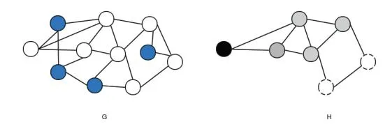
Fig. 1. Graph partition: G is relation graph, and H is vertex-induced graph that is covered by 3 cliques

Algorithm 1 Distribution-Free Learning policy for single-play with side observation (DFL-SSO)

1: For each time slot $t = 0, 1, \dots, n$ Select an arm i by maximizing

$\overline{X}_{i,t} + \sqrt{\frac{\log\left(t/(KO_{i,t})\right)}{O_{i,t}}} \tag{5}$

to pull

2: for $k \in N_i$ do
3: $O_{k,t+1} \leftarrow O_{k,t} + 1$ 4: $\overline{X}_{k,t+1} \leftarrow X_{k,t}/O_{k,t} + (1 1/O_{k,t})\overline{X}_{k,t}$
5: end for
6: end for

graph to rewrite regret in terms of cliques, and then mainly tighten the upper bound by analyzing regret of cliques.

1. Partition relation graph and rewrite regret of subgraph H in terms of cliques.

We order the arms in an increasing order of $\Delta_i$ . We use $\Delta_{c_0} \leq \delta_0 = \alpha \sqrt{K/n} \leq \Delta_{c_0+1}$ to split the K arms into two disjoint sets, one set $K_1$ with $\Delta_x \leq \Delta_{c_0}$ and the other set $K_2$ with $\Delta_x > \Delta_{c_0}$ (We will set the value of $\alpha$ in later analysis). Let $c_0$ be the smallest index of arm satisfying $\Delta_k \leq \Delta_{c_0}$ . We remove all arms in $K_1$ from the relation graph G, as well as adjacent edges to nodes in $K_1$ . In this way, we get a subgraph H of G, over arms in $K_2$ . The regret satisfies,

$\Re(n) \le n\Delta_{c_0} + \Re_H(n),\tag{7}$

where $\mathfrak{R}_H(n)$ is regret generated by selecting suboptimal arms in $K_2$ .

Consider a clique covering C of H, i.e., a set of cliques such that each $c \in \mathcal{C}$ is a clique and $V = \bigcup_{c \in \mathcal{C}} c$ . We define the clique regret $\mathfrak{R}_c(n)$ for any $c \in \mathcal{C}$ by

$\mathfrak{R}_c(n) = \sum_{t < n} \sum_{i \in c} \Delta_i \mathbf{1} \{ I_t = i \}.$ (8)

Since the set of cliques covers the whole graph H, we have

$\mathfrak{R}_{H}(n) \le \sum_{c \in \mathcal{C}} R_{c}(n). \tag{9}$

We give an illustration of the partition process in Fig. 1, where the relation graph G contains one small set of blue nodes representing $K_1$ with $\Delta_i$ below $\Delta_{c_0}$ , and the other large set of white nodes denoting $K_2$ with $\Delta_i$ above $\Delta_{c_0}$ . The vertex-induced subgraph H of $K_2$ is covered by a minimum of 3 cliques, respectively marked by black, gray and dash lines.

2. Regret analysis for regret of subgraph H

In the rest part, we focus on proving upper bound of regret $\mathfrak{R}_H(n)$ . Let $\Delta_c = \max_{i \in c} \Delta_i$ , and $T_c(t) = \sum_{i \in c} T_i(t)$ denote the number of times (any arm in) clique c has been played up to time t, where $T_i(t)$ is the number of times arm i has been selected up to time t. Similarly, we suppose that cliques are ordered in the increasing order of $\Delta_c$ . Let $v_j = \mu_1 - \frac{\Delta_j}{2}$ for cliques in $K_2$ , $c_0 \leq j \leq K$ , and $v_{c_0} = \mu_1 - \frac{\Delta_{c_0}}{2}$ . Let $z_{c_0} = +\infty$ and $\Delta_{K+1} = +\infty$ . For better description, we use $c_0$ to denote the case of c = 0.

As every arms in a clique c must be observed for the same number of times, then for each clique and $l_0 > 0$ , we have

(5) $\Re_c = \sum_{i \in c} \Delta_i T_i(n) \le l_0 \max_{i \in c} \Delta_i + \sum_{i \in C} \sum_{l=l_0}^{\infty} \mathbf{1} \{ I_t = i, t \ge l_0 \}$ (10)

Meanwhile,

$\mathfrak{R}_H(n) = \sum_{c \in K} \mathfrak{R}_c = \sum_{c \in \mathcal{C}} l_0 \Delta_c + \sum_{i=1}^K \Delta_i T_i'(n), \tag{11}$

Where $T_i'(n)$ denotes the number of arm i played after $t = l_0$ , and we refer to the second term as $\mathfrak{R}'_H$

Define

$W = \min_{1 \le t \le n} W_{1,t},\tag{12}$

and

$U_{j,i} = \mathbf{1}_{W \in [v_{j+1}, v_j)} \Delta_i T_i'(n). \tag{13}$

We have the following for $\mathfrak{R}'_H(n)$ ,

$\mathfrak{R}'_{H}(n) = \sum_{i=c_0}^{K} \Delta_i T'_i(n)$ (14)

$= \sum_{j=c_0}^{K} \sum_{i=1}^{j} U_{j,i} + \sum_{j=c_0}^{K} \sum_{i=j+1}^{C} U_{j,i}.$ (15)

For the first term of Equation (15), we have:

$\sum_{j=c_0}^{K} \sum_{i=1}^{j} U_{j,i} \leq \sum_{j=c_0}^{K} \mathbf{1}_{W \in [v_{j+1}, v_j)} n \Delta_j$ (16)

$= n\Delta_{c_0} + n\sum_{c=1}^{C} \mathbf{1}_{W \le v_c} (\Delta_c - \Delta_{c-1}) (17)$

We have the first equation as $\Delta_i \geq \Delta_i$ and $T_i \leq n$ . To bound the second term of Equation (15), we record

$\tau_i = \{ \min t : W_{i,t} < v_i \}$ (18)

after $l_0$ . To pull a suboptimal arm i at t, one must have $W_{i,t}$ $W_{1,t} \geq W$ . By Algorithm 1, we have $\{W \geq v_i\} \subset \{T'_i(n) \leq v_i\}$ $\tau_i$ }, since once we have pulled $\tau_i$ times arm i its index will always be lower than the index of arm 1.

Therefore, we have

$\Re(n) \leq 2n\Delta_{c_0} + \sum_{c \in \mathcal{C}} l_0 \Delta_c + \sum_{i=1}^K \Delta_i \mathbf{E}(\tau_i | t > l_0)$

$+ n \sum_{c=1}^{\mathcal{C}} \mathbf{1}_{W < v_c} (\Delta_c - \Delta_{c-1}). \tag{19}$

For any $l_0 > 0$ ,

$\Delta_{i} \mathbf{E}(\tau_{i} | \tau_{i} > l_{0}) \tag{20}$

$\leq \sum_{l=l_{0}}^{+\infty} \mathbf{P}(\tau_{i} \geq l)$

$= \sum_{l=l_{0}}^{+\infty} \mathbf{P}(\forall t \leq l, W_{i,t} > v_{i})$