Nonparametric Pricing Bandits Leveraging Informational Externalities To Learn The Demand Curve

Abstract. We propose a novel theory-based approach to the reinforcement learning problem of maximizing profits when faced with an unknown demand curve. Our method, rooted in multiarmed bandits, balances exploration and exploitation across various prices (arms) to maximize rewards. Traditional Gaussian process bandits capture one informational externality in price experimentation—correlation of rewards through an underlying demand curve. We extend this framework by incorporating a second externality, monotonicity, into Gaussian process bandits by introducing monotonic versions of both the Gaussian process-upper confidence bound and Gaussian process-Thompson sampling algorithms. Through reduction of the demand space, this informational externality limits exploration and experimentation, outperforming benchmarks by enhancing profitability. Moreover, our approach can also complement methods such as partial identification. Additionally, we present algorithm variants that account for heteroscedastic noise in purchase data. We provide theoretical guarantees for our algorithm and empirically demonstrate its improved performance across a broad range of willingness-to-pay distributions (including discontinuous, time varying, and real world) and price sets. Notably, our algorithm increased profits, especially for distributions where the optimal price lies near the lower end of the considered price set. Across simulation settings, our algorithm consistently achieved over 95% of the optimal profits.

1. Introduction

We propose a new method based on reinforcement learning using multiarmed bandits (MABs) for pricing by efficiently learning an unknown demand curve. Our algorithm is a nonparametric method that incorporates microeconomic theory into Gaussian process (GP)- Thompson sampling (TS). Specifically, we impose weak restrictions on the monotonicity of demand, creating informational externalities between the outcomes of arms in the MAB. Our method exploits these informational externalities to achieve more efficient experimentation and higher profitability, and it enables more flexible price sets than current methods.

Consider a manager tasked with determining the price for a product or service. A natural starting point is to use knowledge of the demand curve. However, the demand curve is typically known only within the limited price range where an established product has been sold, leaving it unknown elsewhere. Consequently, pricing errors are most pronounced for new products that differ significantly from past offerings (Huang et al. 2022). Even in well-established categories, demand can change substantially across markets and time. A global survey of sales vice presidents, chief marketing officers, and chief executive officers at more than 1,700 companies conducted by Bain & Company highlights the insidious impact of poor pricing, which can cause long-term and persistent damage to a firm’s financial prospects (Kermisch and Burns 2018).

To learn the demand curve, a common approach is A/B experimentation (Furman and Simcoe 2015), which randomly allocates consumers across a set of different prices, typically in a balanced experiment. However, this approach presents several challenges.

^*Corresponding author

First, firms across a wide range of industries are often reluctant to conduct extensive price experimentation because of frictions (Aparicio and Simester 2022) or risks. For example, price experimentation can confuse consumers or alter their expectations, leading to uncertain gains (Dholakia 2015).1 Second, firms often do not run experiments for long-enough durations, making it difficult to detect effects (Hanssens and Pauwels 2016). Third, even in well-known categories, demand can undergo significant changes over time, necessitating periodic relearning of demand.

These factors directly imply that a method capable of efficiently identifying and learning the critical part of the demand curve with minimal experimentation can be highly valuable, particularly for identifying the optimal price points for products. This problem is especially suited to a reinforcement learning method known as multiarmed bandits, which simultaneously learn while earning, thereby avoiding the wasteful explorations associated with A/B testing. MABs address the classic trade-off between exploitation (maximizing current payoff) and exploration (gathering additional information) as the agent seeks to maximize rewards over a given horizon.

Two common MAB algorithms are upper confidence bound (UCB) and Thompson sampling. The UCB algorithm (Auer 2002, Auer et al. 2002) constructs an upper confidence bound for the reward of each arm by combining the estimated mean reward with an exploration bonus. This balance between exploiting high-payoff arms and exploring less certain ones is achieved by selecting the arm with the highest upper confidence bound. Meanwhile, the TS approach involves Bayesian updating of the reward distribution for each arm as they are played (Thompson 1933). Arms are chosen probabilistically, with those having higher means being more likely to be selected. Thus, TS is a stochastic approach, whereas UCB is deterministic.

One notable feature of UCB and TS is that they treat the rewards from arms as independent. However, in pricing, this assumption does not hold as an underlying demand curve connects the different arms (prices). In this paper, we propose a new MAB method that builds upon canonical bandits by leveraging two distinct but related sources of informational externalities informed by economic theory on demand curves.

The first informational externality that we observe is that rewards are correlated across prices through the demand function. Specifically, demand at closer price points is more likely to be similar than demand at more distant points. This means that the demand at a focal price point provides insights not only about that price but also, about others. This relationship has been previously recognized in the bandit literature and implemented using a Gaussian process combined with baseline bandit methods (Ringbeck and Huchzermeier 2019). Modeling demand with a GP allows for the learning of a more general reward function rather than restricting learning to rewards associated with specific arms. We empirically build on this research through a systematic study of its impact across various settings.

The second informational externality is the characterization that aggregate demand curves are monotonic, consistent with microeconomic theory. Specifically, the quantity demanded at a focal price must be weakly lower than the demand at all prices below the focal price. However, imposing monotonic shape restrictions in the GP space is not trivial; addressing this challenge constitutes the main contribution of our paper. We leverage the idea that sign restrictions are easier to impose. The connection between the two is established by noting that (i) a monotonically decreasing function is equivalent to its first derivative being negative at every point and (ii) the derivative of a GP is also a GP. Critically, this transforms the problem from imposing monotonic shape restrictions in the original GP space to imposing sign restrictions in the GP space of derivatives.

We make the following contributions. To researchers and practitioners, we provide a method that builds upon Gaussian process bandits by specifying demand curves to be downward sloping without parametric restrictions. Our algorithm efficiently obtains only monotonic, downward-sloping demand curves throughout the price experimentation process. We demonstrate the effectiveness of the algorithm through theoretical analysis and by evaluating performance relative to benchmarks for a wide range of conditions, including from field data. Our approach results in significantly higher profits relative to state-of-the-art methods in the MAB literature. Furthermore, we characterize the underlying willingness-to-pay (WTP) distributions under which our algorithm delivers greater performance improvements and explore the mechanisms driving these results. Overall, the increase in efficiency means that a larger number of prices can be included in the consideration set. These are important managerial considerations given the frictions in undertaking pricing experimentation. More broadly, in other situations where data have some general known form a priori, our approach shows how such constraints can be combined with the flexibility of nonparametric bandits to improve empirical performance.

Our method offers several advantages relative to existing approaches for optimal pricing under unknown demand. The primary advantage is its efficiency in achieving optimal pricing by learning demand in a flexible, nonparametric manner, particularly when the firm lacks well-defined prior information. If a firm is willing to undertake adaptive experimentation to learn demand while minimizing the cost of experimentation, our method enables the firm to achieve higher profitability. A second advantage is the method’s ability to systematically incorporate theoretical knowledge into reinforcement learning problems, ensuring that the resulting demand satisfies theoretical constraints. Furthermore, it can be applied to learn about consumer valuations for any vertical quality-like attribute, not just prices. Third, our method provides an estimate of uncertainty in addition to point estimates of the demand curve. Indeed, the entire posterior distribution can be obtained, offering a complete characterization of uncertainty around the learned demand curve. Importantly, this approach also provides demand estimates for prices outside the initial price set chosen. Fourth, the method requires little to no human judgment. Unlike most typical reinforcement learning models, hyperparameter tuning is automatic, and the method is computationally tractable, allowing the bandit to operate in real time. Fifth, our method does not rely on any knowledge of consumer characteristics unlike partial identification approaches such as upper confidence bound with partial identification (Misra et al. 2019). It can, however, be used in conjunction with partial identification methods to enhance performance.

We derive theoretical regret bounds for GP-TS when monotonicity is incorporated. Our analysis follows the standard approach of Srinivas et al. (2009) and achieves similar results. However, by enforcing monotonicity, the space of feasible demand curves is reduced, which in turn, decreases the path-dependent regret term and results in tighter regret bounds.

Empirically, we run simulations across a range of settings and find that our proposed algorithm outperforms several state-of-the-art benchmarks, including UCB, TS, nonparametric Thompson sampling (N-TS), GP-UCB, and GP-TS. Averaged across three main underlying willingness-to-pay distributions, our algorithm achieves the highest performance, reaching 92% of optimal profits after 500 consumers and 97% of optimal profits after 2,500 consumers. Furthermore, we observe that profits consistently increase when monotonicity is incorporated into GP-UCB (by 20%–26% after 500 consumers and 5%–8% after 2,500 consumers) and GP-TS (by 9%–13% after 500 consumers and 4%–5% after 2,500 consumers), regardless of the price set granularity (number of arms). However, there is substantial heterogeneity in the observed uplifts depending on the underlying distribution. The largest gains occur when the optimal price lies near the lower end of the price set. This variation in uplifts is driven by heterogeneity in benchmark performance across underlying distributions, whereas our algorithm performs consistently.

We also test additional challenging scenarios. First, we evaluate the case where demand exhibits a discontinuity motivated by the left-digit bias, which presents a challenge because a GP assumes continuity. We find that our proposed method continues to perform best. However, if managers are particularly concerned about a sufficiently large left-digit bias, they may wish to focus only on prices at the discontinuities. Next, we consider cases where long-term advantages might arise from using our method. Specifically, we examine situations where demand varies with seasonality and find that even when these shifts are unpredictable, our proposed method achieves a long-run performance advantage over the benchmarks. Further, we demonstrate that these advantages persist in real-world settings using a valuation distribution estimated from data on demand for a streaming service. Finally, we develop an alternative specification that accounts for heteroscedastic noise in the purchase input data, resulting in small additional performance gains.

2. Literature Review

Our research is related to several streams detailed below. The setting features pricing experimentation and learning over time, which are active areas of research across marketing, operations research, economics, and computer science.

2.1. Demand Learning

Studies in marketing and economics typically make strong assumptions about the information that a firm has regarding product demand. The strongest assumption used is that the firm can make pricing decisions based on knowing the demand curve (or willingness to pay) (Oren et al. 1982, Rao and Bass 1985, Tirole 1988). A generalization of this assumption is that firms know the demand only up to a parameter, as in earlier works on learning demand through price experimentation (Rothschild 1974, Aghion et al. 1991). Extending this idea beyond a single parameter, much of the subsequent literature specifies a consumer utility function in terms of product characteristics, price, and advertising, with preference parameters estimated from data (Jindal et al. 2020, Zhang and Chung 2020, Huang et al. 2022). However, all of these models predetermine the shape of the demand curve and cannot incorporate all possible demand curves. Nonparametric approaches are the gold standard and have been used to account for state changes between periods, but they are often simplified substantially (e.g., having two periods) to ensure analytical tractability (Bergemann and Schlag 2008, Handel and Misra 2015). However, this stream typically does not consider learning through active experimentation, which is the focus of multiarmed bandits stream below.

2.2. Multiarmed Bandits

Multiarmed bandit methods are an active learning approach based on reinforcement learning and are used across many fields, with business applications in advertising (Schwartz et al. 2017), website optimization (Hauser et al. 2009, Hill et al. 2017), and recommendation systems (Kawale et al. 2015). Two fundamental arm selection algorithms (or decision rules) that form the foundation for MAB methods are (a) upper confidence bound based on Auer et al. (2002), which is a deterministic approach, and (b) Thompson sampling based on Thompson (1933), which is a stochastic approach.

Several previous works have explored dynamic pricing with nonparametric demand assumptions. These often enforce conditions, like smoothness or unimodality, and then, approximate the demand using locally parametric functions, such as polynomials (Wang et al. 2021). However, the resulting algorithms depend heavily on these specific choices. In contrast, our approach imposes no constraints beyond the economically motivated monotonic shape constraint. Any further restrictions arise naturally from the chosen kernel (e.g., radial basis function (RBF) or Matern), offering greater flexibility for practitioners hesitant to make strong assumptions.

Although shape constraints have been considered in other contexts, their application to pricing and reward maximization remains limited. Thresholding bandits aim to find the arm closest to a given threshold, assuming monotonic arm rewards, but they do not focus on maximizing rewards (Cheshire et al. 2020). Other works primarily address the estimation problem (Guntuboyina and Sen 2018) or consider contextual settings with monotonic mean distributions across arms (Chatterjee and Sen 2021). These approaches, although valuable, do not directly translate to our pricing problem with a focus on reward maximization under shape constraints motivated by economic theory.2

However, traditional bandit methods typically only model rewards for individual arms but not any dependencies across arms. In pricing applications, this independence ignores the information from the underlying demand curve, which we term as informational externalities. Recent research below has tried to develop methods to address this issue.

2.2.1. Gaussian Processes and Bandits. Gaussian processes are well regarded as a highly flexible nonparametric method for modeling unknown functions (Srinivas et al. 2009). GPs provide a principled approach to allowing dependencies across arms without restricting the functional form. Multiarmed bandits combining GPs along with a decision rule, like UCB or Thompson sampling, have been proposed (Chowdhury and Gopalan 2017).

More specifically, a closely related paper by Ringbeck and Huchzermeier (2019) uses GP-TS for a multiproduct pricing problem. The GP is modeled here at a demand level, which is important for two reasons. First, it allows for modeling demand-level inventory constraints in a multiproduct setting, and second, it allows for a separation of the learning problem (at the demand level) from the rewards optimization (reward is the product of demand and price). Leveraging the first informational externality, they find that GP-TS improves performance over TS. However, much is not known about the conditions (e.g., the number of arms or WTP distribution or stability of the demand curve) under which the informational externality modeled by GP-TS is important, with a material impact on profit outcomes. Our focus here is on incorporating monotonicity of demand curves, a theory-based restriction that forms the second informational externality, into GP-TS and GP-UCB models and evaluating the resulting models. We also evaluate the value of these informational externalities across a wide spectrum of conditions.

There are other approaches to ruling out dominated prices (arms) in pricing bandits. One particularly notable contribution that incorporates knowledge into bandits is the partial identification method (Misra et al. 2019). Although this approach leverages weakly decreasing demand curves, it does not otherwise rely on dependencies across arms. Partial identification formalizes the idea that the rewards from a specific arm (price) can be dominated by those of another arm and critically depends on the availability of highly informative segmentation data to estimate demand bounds for each segment. These demand bounds are then aggregated across all segments to derive the corresponding aggregated reward bounds for each price. Dominated prices are eliminated if the upper bound for one price is lower than the lower bound for another price. In contrast, our algorithm does not require segmentation data to exploit the gains from the monotonicity assumption. Because the mechanisms in these approaches differ, partial identification can complement our method, enabling the creation of a hybrid approach.

3. Pricing Problem and Simple Example 3.1. Pricing Problem

We address the pricing problem faced by a firm aiming to maximize cumulative profits while experimenting under an unknown demand curve. Potential buyers (consumers) arrive sequentially and are presented with a price selected by the firm. Each consumer then decides whether to purchase a single unit or not (in line with Misra et al. 2019, we focus on discrete choice purchases) depending on whether the offered price is below or above their willingness to pay.3 For each consumer, the reward (profit) received by the firm equals the price minus the cost if the consumer makes a purchase and zero otherwise.

Overall, the firm must make two key decisions. First is the selection of the set of prices to be tested in the experiment; this is assumed to be exogenous, although in our simulations, we test multiple price sets with varying granularities to guide firms in this decision. Second, the firm is allowed to periodically adjust the price shown to an incoming consumer based on limited past purchase decisions obtained during the pricing experiment. This paper focuses on designing an algorithm that selects prices (from the price set) throughout the experiment to maximize profits. The algorithms considered belong to a class known as multiarmed bandits described in Section 4.

We consider a few additional assumptions in this pricing problem. First, consumers are randomly drawn from a population with a stable WTP distribution of valuations. Second, consumers are short lived, and the overall distribution of price expectations remains unaffected by the experimentation. These assumptions are typical in field experiments and necessary for the results to be applicable once the experiment has ended. Third, we assume that the firm operates as a single-product monopolist.⁵ Fourth, the firm seeks to set a single optimal price, meaning that it does not engage in price discrimination and does not consider inventory or other factors (Besbes and Zeevi 2009, Ferreira et al. 2018, Misra et al. 2019, Ringbeck and Huchzermeier 2019).6 Finally, given the pace at which prices must be adjusted for efficient experimentation, our algorithms are suited to the online domain rather than physical stores.

3.2. Simple Pricing Experiment Example

We now illustrate a simple example of a balanced pricing experiment with certain valuation distributions to show why existing bandit algorithms may struggle and how our algorithm can enhance performance. Consider a monopolist firm selling a single-unit product of zero marginal cost who tests prices $P = \{0.1, 0.3, 0.5, 0.7, 0.9\}$ each 100 times; they face an unknown demand curve D(p) = 1 - p. Figure 1 presents the results of demand and profit learning. Figure 1(a) shows sample mean demand at tested prices (blue dots) with 95% credible intervals, whereas Figure 1(b) displays sample mean profit (red dots) with 95%

credible intervals. Grey dotted lines in Figure 1 represent the true demand and profit curves.

Figure 1 highlights a key phenomenon; the credible intervals for demand are fairly consistent,7 but those for profit vary greatly and expand with price because of the scaling effect. Learning occurs at the demand level, but optimal pricing decisions depend on profit. Consequently, the difficulty of identifying the optimal price depends on its position within the tested prices. A high optimal price simplifies the task as learning that lower prices yield smaller profit intervals is less challenging. Conversely, a low optimal price complicates the task as determining that higher prices are suboptimal requires more consumer purchase data. This results in poorer algorithmic performance when the optimal price is low. Incorporating monotonicity enhances performance by excluding any demand curve where demand increases with price, thereby narrowing the range of possible demand curves and reducing demand intervals. This effect is amplified by the scaling effect, significantly lowering the profit intervals at high prices.

4. Model Preliminaries

4.1. MAB Components

This section formally introduces multiarmed bandits and their application to the pricing problem. Notably, all MABs have three components: actions, rewards, and a policy.

The first component—actions—refers to the set of prices from which the firm can choose. Prior to the experiment, the firm selects a finite set of A ordered prices $P = \{p_1, \ldots, p_A\}$ , where $p_1 < p_2 < \cdots < p_A$ , and prices are scaled so that $0 \le p_a \le 1$ .⁸ Although this paper does not

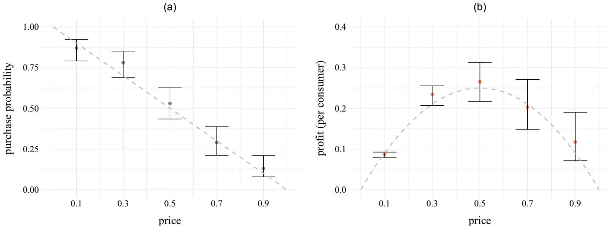
Notes. Results are shown of a single balanced experiment where each of the prices $\{0.1, 0.3, 0.5, 0.7, 0.9\}$ was tested 100 times with a true unknown demand of D(p) = 1 - p. Panel (a) shows the means and 95% credible intervals for purchase probability at each price tested; the dotted gray line shows the true purchase probability. Panel (b) shows the means and 95% credible intervals for profit at each price tested; the dotted gray line shows the true expected profit. (a) Demand learning. (b) Profit learning.

explicitly model how to choose the set of prices, the general trade-off is that learning is easier with fewer prices, but a higher optimum is possible when more prices are considered. Section 6.5 provides general guidelines for how to pick the set of prices. Once P is chosen, at each time step t of the experiment, the firm chooses a price $p_a$ from P.

The second component—rewards—refers to the profits that a firm makes at each purchase opportunity. The firm faces an unknown true demand D(p), and the true profit function is given by $\pi(p) = pD(p)$ . We assume that variable costs are zero, although the model can easily accommodate such costs. The true profit is not observed; instead, the firm observes noisy realizations of profits corresponding to each price $p_a$ . Considering the data at each price separately, we define $n_{at}$ to be the number of times that price $p_a$ has been chosen through time t and $s_{at}$ to be the cumulative number of purchases for action a through time t. The observed purchase rate through time t for price $p_a$ is simply $y_{at} = \frac{s_{at}}{n_{at}}$ . Accordingly, the mean profit for a price $p_a$ at time t is $\bar{\pi}_{at} = p_a(\frac{s_{at}}{n_{at}})$ .

The final component—a policy—denoted by $\Psi$ is a decision-making rule that picks an action or price in each round using the history from past rounds. In this situation, the history can be written as $H_t = \{S_t = (s_{1t}, \ldots, s_{At}), N_t = (n_{1t}, \ldots, n_{At})\}$ . Formally, in round t, the policy picks a price using the history from the past (t-1) rounds: $p_{a_t} = \Psi(P, H_{t-1})$ . What distinguishes various MAB algorithms is how this policy is defined. For a typical randomized experiment, the policy can be defined as an equal probability across all arms, completely ignoring history. A summary of the notation is given in Table 1.

4.2. Performance Metrics

To assess the performance of our proposed algorithm, we need to compare it with other bandit algorithms. This is equivalent to a comparison of policies as only the

policy $\Psi$ depends on the algorithm, whereas the price set and arm rewards are common across algorithms.

Among the various performance metrics in the bandit literature, the most common is regret, which is defined as the difference between rewards under full knowledge (always playing the optimal price) and the expected rewards from the policy in question (Lai and Robbins 1985). Formally, the cumulative regret of policy $\Psi$ through time t is

$\operatorname{Regret}(\Psi, P, t) = \mathbb{E}\left[\sum_{\tau=1}^{t} (\pi^* - \pi_{a_{\tau}} | \Psi, P, H_{\tau-1})\right], \quad (1)$

where P is the set of prices being considered, $\pi^*$ is the ex post maximum expected profit in a given round, and $\pi_{a_{\tau}}$ is the profit realized when price $p_a$ is played in time period $\tau$ . This metric¹⁰ is used in the discussion of theoretical properties in Online Appendix EC.4.¹¹

An alternative objective is to maximize the expected total reward (Gittins 1974, Cohen and Treetanthiploet 2020). Tormally, the goal is to pick a decision rule, $\Psi$ , that selects a sequence of prices from the consideration set, P, that maximizes the total expected profit:

\mathbb{E}\left[\sum_{\tau=1}^{t} \pi_{a_{\tau}} | P\right]. \tag{2}

We use this metric to discuss our empirical simulation results as it is more intuitive in the context of the pricing problem (a firm maximizing profits through experimentation with an unknown demand curve). Additionally, if the true rewards distribution is unknown (e.g., in a field experiment), total rewards can still be compared, whereas regret lacks a straightforward alternative formulation.

4.3. Baseline Policies—Deterministic and Stochastic Algorithms

Finally, we consider baseline policies, which serve as building blocks for our algorithm. The simplest approach

Table 1. Summary of Bandit Notation

Notation $\Psi$	Description Pricing policy (i.e., decision rule)	Formula Depends on the algorithm
a t	Action from the set of actions $\mathcal{A}$ Time step; denotes the $t$ th consumer of the price experiment	$a \in \mathcal{A} = \{1, 2, \dots, A\}$
$P$ $p_a$ $n_{at}$ $s_{at}$	Set of prices to be tested Scaled price corresponding to action $a$ Number of times that price $p_a$ has been chosen through time $t$ Number of purchases at price $p_a$ through time $t$	$p_a \in P = \{p_1, \dots, p_A\}, \text{ where } 0 \le p_a \le 1 \ \forall p_a$
$H_t$ $a_t$ $D(p_a)$ $y_{at}$	History from past $t$ rounds of the experiment Action chosen at time $t$ Demand at price $p_a$ Purchase rate through time $t$ of price $p_a$	$H_t = \{S_t = (s_{1t}, \dots, s_{At}), N_t = (n_{1t}, \dots, n_{At})\}$ $a_t = \Psi(P, H_{t-1})$ $y_{at} = s_{at}/n_{at}$
$ar{\pi}_{at}$ $\pi_{a_t}$	Mean profit through time $t$ of price $p_a$ Profit realized when price $p_a$ was tested in time period $t$	$\bar{\pi}_{at} = p_a(s_{at}/n_{at})$

is a fully randomized experiment (A/B testing), where a random arm is selected, ignoring the history of arms played and their outcomes. Another class includes myopic policies, such as greedy-based algorithms (e.g., $\epsilon$ -greedy) and softmax (Dann et al. 2022). In this paper, we build on two popular policies, UCB and TS, which trade off learning and earning and form a fundamental component of typical bandit algorithms.

4.3.1. UCB. The upper confidence bound algorithm is a deterministic, nonparametric approach popularized for its proven asymptotic performance, achieving the lowest possible maximum regret (Lai and Robbins 1985, Agrawal 1995, Auer et al. 2002). The UCB policy scores each arm by summing an exploitation term and an exploration term and then selecting the arm with the highest score. The exploitation term is the sample mean of past rewards at a given arm, which provides information about past payoffs. The exploration term, meanwhile, increases with the uncertainty of the sample mean for an arm; specifically, it decreases as an arm is chosen more frequently and as the empirical variance of rewards at that arm decreases. Thus, the UCB policy balances exploitation and exploration.¹³ To adapt UCB to pricing, we scale the exploration term by price (Misra et al. 2019) as shown in Equation (3). This adjustment accounts for the known variation in the range of possible rewards at each arm, which is not generally assumed:

$p_a^{\text{UCB}} = \arg\max_{p_a \in P} \left( \bar{\pi}_{at} + p_a \sqrt{\frac{\log(t)}{n_{at}}} \min\left(\frac{1}{4}, V_{at}\right) \right)$

$V_{at} = \left(\frac{1}{n_{at}} \sum_{\tau=1}^{n_{at}} \pi_{a\tau}^2 \right) - \bar{\pi}_{at}^2 + \sqrt{\frac{2\log t}{n_{at}}}.$ (3)

4.3.2. TS. Thompson sampling is a randomized Bayesian parametric approach. For each arm, a reward distribution is specified with a prior and updated based on the history of past trials (Thompson 1933). In each round, an arm is chosen according to the probability that it is optimal given the history of past trials. Specifically,

$Prob(p_a|H_{t-1}) = Prob(E[\pi_{a,t}|p_a] > E[\pi_{a,t}|p_{a'}], \forall p_{a'} \neq p_a|H_{t-1}).$ (4)

The simplest implementation is to sample from each distribution in each round and select the arm with the highest sampled payoff. In our setting, where purchase decisions are binary, the TS approach uses a scaled Beta distribution, with parameters representing the numbers of successes and failures (Chapelle and Li 2011, Agrawal and Goyal 2012). Specifically, at time t+1 for each arm a, a sample is drawn from Beta( $s_{at}+1$ , $n_{at}-s_{at}+1$ )

and then scaled by the price, $p_a$ . The arm with the highest value is then chosen.

Another benchmark we consider is nonparametric Thompson sampling by Urteaga and Wiggins (2018), which extends standard TS to handle reward model uncertainty. Unlike traditional TS, which requires knowledge of the true reward model, N-TS uses Bayesian nonparametric Gaussian mixture models to flexibly estimate each arm’s reward distribution. This approach allows the complexity of the per-arm reward model to adjust dynamically as new observations are collected, enabling sequential learning and improved decision making.

5. Informational Externalities

In this section, we incorporate the two informational externalities into the baseline policies. Our objective is to create a general method that combines any decision rule (such as UCB, TS, or others) with the two relevant informational externalities. The first informational externality—continuity—is implemented using Gaussian process bandits developed by Srinivas et al. (2009). The main contribution of this paper, however, is the incorporation of the second externality—monotonicity—which also builds on the Gaussian process framework. An overview of how these externalities are incorporated into the baseline policies is shown in Figure 2.

5.1. First Informational Externality: From Points to Functions

The first informational externality recognizes the local dependence of functions through continuity, whereas baseline MABs consider outcomes at discrete arms to be separate and independent. Specifically, in the pricing application, we know that demands at two prices tend to be closer when the prices are closer together. With 10 arms, to inform demand at arm a (say price $p_a = 0.5$ ), the demands at $p_{a-1} = 0.4$ and $p_{a+1} = 0.6$ are

Figure 2. (Color online) Overview of the Incorporation of Informational Externalities

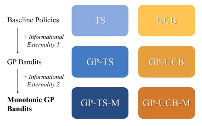
Note. GP-TS-M, monotonic version of Gaussian process-Thompson sampling; GP-UCB-M, monotonic version of Gaussian process-upper confidence bound.

most informative. More generally, it is possible to learn about the demand D(p) at price p from observed demands at nearby price points, such as $D(p+\epsilon)$ for small $\epsilon$ . Note that the information spillover is bidirectional, with points farther away being less important and weighted less because of the structure of the covariance matrix.

The logic of sharing information between arms means that using functions to model demand across the range of prices, rather than focusing only on demand at specific arms (price points), may lead to increased performance. A straightforward parametric approach would involve specifying functional forms (e.g., splines) to flexibly model the true demand curve using observations at the arms (prices). However, there is a risk that any parametric approximation chosen by the researcher may be insufficient to capture the true shape of the demand curve.

We take a more flexible nonparametric approach by modeling the space of demand functions as a Gaussian process. A Gaussian process is a stochastic process (a collection of random variables) such that every finite subset has a multivariate Gaussian distribution; a simple example of fitting a GP to data can be found in Online Appendix EC.1. GPs can be thought of as a probability distribution over possible functions, allowing any function to be probabilistically drawn from the function space on the chosen support, unlike typical parametric models. Thus, any arbitrary demand curve can be modeled, and the GP learns the shape from the data. Following Srinivas et al. (2009), GPs can be incorporated into the bandit framework using both UCB and TS (Chowdhury and Gopalan 2017).

5.1.1. Advantages of GPs Relative to Other Methods.

GPs offer several desirable features for the present class of problems. First, GPs provide a parsimonious, nonparametric approach to incorporating both informational externalities in a transparent, principled, and provable manner. Second, GPs have closed-form solutions that allow hyperparameters to be tuned quickly with maximum likelihood estimation. Intuitively, GPs work well with bandits because the exploration-exploitation trade-off relies on understanding the complete distribution of rewards, not just the mean reward at each arm. A GP, which specifies a probability distribution over functions, offers a principled way to manage the exploration-exploitation trade-off.

Finally, we note that other nonparametric methods, including many machine learning methods, may provide higher-accuracy estimates for the mean. However, because they are not typically capable of quantifying the certainty of their predictions, they are ill suited for bandit algorithms, where managing the exploration-exploitation trade-off is crucial. In contrast, GPs directly quantify uncertainty, allowing it to

be incorporated into the decision-making process in a principled way. If only the means of the posterior GP are used (thus ignoring model uncertainty), algorithmic performance has been shown to decrease (Srinivas et al. 2009). ¹⁶

5.1.2. Gaussian Processes. The key building block of our approach, which underpins the modeling of both informational externalities, is the Gaussian process. As in Ringbeck and Huchzermeier (2019), we model the GP at the demand level and then scale by price, allowing the bandit to make decisions at the reward level. A summary of the GP notation we use is provided in Table 2.

5.1.2.1. Training Data. The goal of estimating a GP is to learn the space of demand functions at test points, P,¹⁷ given the purchase decision history obtained at time t from the MAB experiment. The training data are defined as $\mathcal{D}_t = \{P_t, y_t\}$ , where $P_t = \{p_a : a \in \mathcal{A}_t\}$ and $y_t = \{y_{at} : a \in A_t\}$ . Here, $A_t \subseteq A$ is the subset of actions tested by time t, and $y_{at} = \frac{s_{at}}{n_{at}}$ represents the observed purchase rate for price $p_a$ at time t. The purchase rates, $y_{at}$ , provide a noisy signal of the true value of the demand function D(p) at $p_a$ ; specifically, we assume $y_{at} = D(p_a) + \epsilon$ , where $\epsilon \sim \mathcal{N}(0, \sigma_{y_a}^2)$ . The vector $\sigma_y^2 = (\sigma_{y_1}^2, \sigma_{y_a}^2)$ …, $\sigma_{\nu_A}^2$ ) is referred to as the noise hyperparameter. Importantly, the cardinality of the training data depends on the number of prices in the test set, |P| = A. Therefore, it does not depend on t, the number of purchase decisions observed, reducing the dimensionality. The computation and equivalence of these two approaches are discussed in Online Appendix EC.2.

5.1.2.2. Kernel. A Gaussian process flexibly models dependencies across input points using a kernel, implemented through a covariance function. A kernel $k(\cdot, \cdot)$ takes two points (in our setting, prices $p_i$ and $p_j$ ) from the input space and returns a scalar representing the covariance between the outputs at those points. From this, a covariance matrix $K(\cdot, \cdot)$ can be constructed for a set of inputs.

A commonly used and robust kernel for GPs is the radial basis function kernel, also known as the

Table 2. Summary of GP Notation

Description	Notation in pricing setting
Training data	$\mathcal{D}_t = \{P_t, y_t\}$
Noise hyperparameter	$\sigma_y^2$
RBF kernel	$k^{\text{RBF}}(p_i, p_j) = \sigma_D^2 e^{\frac{-(p_i - p_j)^2}{2l^2}}$
RBF hyperparameters	$\{\sigma_D, l\}$
Covariance function (kernel) evaluated at two points	$k(p_i,p_j)$
Covariance matrix between price vectors	K(P,P)

Gaussian kernel or the squared exponential kernel (Duvenaud 2014):

$k^{\text{RBF}}(p_i, p_j) = \sigma_D^2 e^{-\frac{(p_i - p_j)^2}{2l^2}}.$ (5)

The RBF kernel has a set of desirable properties suited to our setting. It is differentiable and can provably approximate any arbitrary continuous target function uniformly on any compact subset of the input space (Micchelli et al. 2006).

5.1.2.3. Shape Hyperparameters. The RBF kernel has two shape hyperparameters, $\sigma_D$ and l. The first hyperparameter, $\sigma_D$ , is a scale factor that controls the amplitude of the function (i.e., the average distance of the function from its mean). The second hyperparameter, l, determines the smoothness¹⁸ of the function, describing how the correlation between two points decreases as the distance between them increases (Shahriari et al. 2015).

A crucial practical step in estimating the GP is tuning the hyperparameters. To minimize human (researcher) judgment, it is ideal to have an efficient, accurate, and automatic method for selecting hyperparameters. We use standard non-Bayesian methods for tuning the hyperparameters.¹⁹ This approach involves choosing values of the hyperparameters that maximize the likelihood of the data given the model. Mathematically, this is equivalent to minimizing the negative log-marginal likelihood (Williams and Rasmussen 2006, equation 2.30):

$\log \text{prob}(y_t|P_t) = -\frac{1}{2}y_t^T (K(P_t, P_t) + \sigma_y^2 I)^{-1} y_t - \frac{1}{2}\log|K(P_t, P_t) + \sigma_y^2 I| - \frac{t}{2}\log(2\pi).$ (6)

5.1.2.4. Noise Hyperparameter. Although the noise hyperparameter can be estimated along with the shape hyperparameters, we choose to specify it directly because of the difficulty of disentangling shape and noise hyperparameters (Williams and Rasmussen 2006).²⁰ A conservative approach to specifying the noise hyperparameter—without estimation is to use the upper bound. We leverage the fact that purchase decisions in our model follow a Bernoulli distribution and lie within the interval [0, 1] to calculate this upper bound, which is 0.25 and occurs when the true purchase probability is 0.5.21 Although this may be overly conservative for some prices, in contrast, setting noise hyperparameters too low could limit exploration and lead to poor results by causing the algorithm to get stuck in errant equilibria. A discussion of alternative methods, where noise takes on different values for different prices (i.e., heteroscedastic noise), is provided in Online Appendix EC.6.

5.1.2.5. Posterior Prediction. Estimating the posterior GP is done using standard GP regression on training data. Equations and an illustrative example are provided in Online Appendix EC.1.

5.1.3. GP-UCB and GP-TS. Gaussian processes can be combined with bandits, such as UCB and TS, to create GP-UCB (Srinivas et al. 2009) and GP-TS (Chowdhury and Gopalan 2017), respectively. The general idea is that instead of using the raw data directly, a posterior GP is estimated before applying a UCB or TS rule to choose a price. As with the baseline algorithms, we scale by price to adapt to the pricing setting.

To initialize the algorithm, we select the first price randomly. Once one data point is available, the training data $\mathcal{D}_t = \{P_t, y_t\}$ can be used to choose the hyperparameters using Equation (6). Additionally, the posterior mean $\mu(D^*)$ and covariance matrix $\operatorname{Cov}(D^*)$ can be calculated using Equations (EC.5) and (EC.6) in the Online Appendix.

With the GP estimated, we can apply either UCB and TS to select a price arm. For GP-UCB, at each price $p_a \in P$ , the posterior demand mean $\mu_t(p_a)$ and variance $\sigma_t^2(p_a)$ are used to determine the price at iteration t+1 according to the following decision rule:

$p_a^{\text{GP-UCB}} = \underset{p_a \in P}{\text{arg max}} (p_a(\mu_t(p_a) + \beta_{t+1}^{1/2} \sigma_t(p_a))),$ (7)

where $\beta_t = \frac{2}{5}\log(|P|t^2\pi^2/(6\delta))$ . Note that we have scaled by $p_a$ as the algorithm is optimizing for reward rather than demand (the level at which the GP was estimated).

On the other hand, in GP-TS, rather than sampling at each arm as in traditional TS, a demand draw for every test price, $D^{(t)}(p_a)$ , can be obtained by sampling from the posterior GP. Specifically, $D^{(t)}(P)$ is a sample from the posterior normal distribution with the given mean and covariance matrix, $D^* \sim N(\mu(D^*), \text{Cov}(D^*))$ . Then, using Thompson sampling, the selected price will be

p_a^{\text{GP-TS}} = \underset{p_a \in P}{\text{arg max}} (p_a D^{(t)}(p_a)). \tag{8}

5.2. Second Informational Externality: Monotonicity

We now focus on the main contribution of this paper: incorporating the second informational externality into Gaussian process bandits. The monotonicity property has a global influence as demand at price $p_j$ , $D(p_j)$ , constrains all demands at higher prices because $D(p_i) \leq D(p_j)$ when $p_i \geq p_j$ . Similarly, all demands at lower prices are constrained as well: $D(p_i) \geq D(p_j)$ when $p_i \leq p_j$ . Note that the impact is asymmetric; specifically, demand at a higher price $p_i$ is upper bounded by demand at a lower price is lower bounded by demand at a higher price.

Our method is general enough to integrate with both GP-UCB and GP-TS as past literature (Chowdhury and Gopalan 2017) shows that neither completely dominates the other. We refer to the monotonic versions of GP-UCB and GP-TS as GP-UCB-M and GP-TS-M, respectively. The goal is to determine whether and under what conditions incorporating monotonicity improves performance for either variant.

When using GP-TS or GP-UCB, the baseline GP allows for any demand function and does not impose any restrictions on the shape. Our goal is to obtain only weakly decreasing monotonic demand functions. For GP-TS-M, we require a way to randomly draw a monotonic function from the set of monotonic functions in the posterior GP. For GP-UCB-M, we require an estimate of the mean and variance from the subset of monotonic demand curves from the posterior; alternatively, this can be approximated by averaging over multiple monotonic draws.

To obtain a random monotonic draw, a simple approach is to use rejection sampling by repeatedly sampling from the GP until a weakly decreasing draw is obtained. Although this approach can work, there is no guarantee that a weakly decreasing draw will be found quickly. This issue is further exacerbated when there are few observations or when there are many test prices; faced with many arms and (noisy) nonmonotonic sample means, the probability of finding a monotonic draw can become vanishingly small.

To ensure that a weakly decreasing draw can be obtained from a GP expediently in all cases, we develop a method from first principles. We note that sampling a monotonic function from a GP is intractable. We, therefore, transform the problem by leveraging a helpful property of GPs that the derivative of a GP is also a GP (and that the RBF kernel is infinitely differentiable), allowing us to estimate the derivative of the GP from our data. The transformed problem, where we obtain a draw from a GP with all values being negative, then becomes a tractable sampling problem (equivalent to sampling from a truncated normal). Specifically, a decreasing monotonic function can be characterized by having negative first derivatives at all points. We then use the basis functions proposed by Maatouk and Bay (2017) to estimate the demand function from a random sample of negative derivatives.

An important property of this principled approach is that the function is guaranteed to be monotonic not only at the discrete price levels forming the support but also at any intermediate price where no experimentation is performed. This ensures consistency in the function’s behavior across the entire price range. The only assumption required is that the demand function is differentiable with a continuous derivative.

5.2.1. Basis Functions. To estimate the demand function, we use a collection of functions $h_j$ known as the interpolation basis. These basis functions are defined a priori and remain the same regardless of the input data. They provide a method for estimating a function at all points by linearly interpolating between known function values at knots spaced over the support. Following Maatouk and Bay (2017), let $u_j \in [0,1]$ for $j = 0,1,\ldots,J$ denote equally spaced knots on [0,1] with spacing $\delta_J = 1/J$ and $u_j = j/J$ . The interpolation basis is defined as

$h_j(p) = h\left(\frac{p - u_j}{\delta_J}\right)$ , where $h(p) = (1 - |p|)\mathbb{1}(p \in [-1, 1])$ .

Then, for any continuous function $D:[0,1] \to \mathbb{R}$ , the function

$D_J(\cdot) \approx \sum_{j=0}^J D(u_j) h_j(\cdot)$ (10)

approximates D by linearly interpolating between function values at the knots $u_j$ . A key property of the interpolation basis is that as the gap between the evenly spaced knots becomes infinitesimally small, the distance between the estimate and the true function converges to zero.

Our goal, however, is to simplify the sampling problem by approximating the demand function in terms of its derivatives at the knot points. Equation (10) can be transformed to express the demand function in terms of its intercept, derivatives, and the original basis functions $h_j$ as shown in Proposition 1 (a derivation is provided in Online Appendix EC.3.2). Online Appendix EC.3.1 provides a visual demonstration of the basis functions $h_j$ and their integrals $\int_0^p h_j(x) dx$ .

Proposition 1. Assuming that a demand function D: $[0,1] \to \mathbb{R}$ is differentiable with a continuous derivative (i.e., $D \in C^1([0,1])$ ), it can be estimated by its intercept and derivatives using the following equation:

$D(p) \approx D(0) + \sum_{j=0}^{J} D'(u_j) \int_0^p h_j(x) dx.$ (11)

Although this approach applies to all class $C^1$ functions on the support, we additionally assume that the unknown demand function D is weakly decreasing, meaning that it belongs to a subset $\mathcal{M}$ defined as follows:

\mathcal{M} := \{ D \in C^1([0,1]) : D'(p) \le 0, p \in (0,1) \}. \tag{12}

In other words, D belongs to the subset of functions where the derivative is never positive at any value of p.

5.2.2. GP-UCB-M and GP-TS-M. There are a few differences between the monotonic and nonmonotonic

versions of GP bandits. When incorporating monotonicity, instead of estimating a GP of the means at the test prices, we first estimate a GP of the derivatives at the knots, concatenated with the mean at the intercept. Crucially, the intercept and derivatives must be estimated together, which is possible because of the property of a GP that the joint distribution of values and their derivatives is also a GP (Online Appendix EC.3.3 provides details on calculating the derivative of a GP). Once the posterior GP is estimated, off-the-shelf sampling can be used to acquire a draw, where every derivative is nonnegative; specifically, we use the TruncatedNormal package in R (Botev and Belzile 2025). Then, Equation (11) provides a formula to recover the demand sample $D^{(t)}$ at the desired test prices using only the draw and basis functions h. From this point, the decision rules for GP-UCB or GP-TS can be applied as usual. Formally, the methods are outlined in Algorithms 1 and 2.

Algorithm 1 (GP-TS-M)

• 1 Set test prices P, kernel k, noise hyperparameter $\sigma_y^2$ , and knots $\mathcal{U}$
• 2 Compute the integrals of the basis functions at U using Equation (9)
• 3 Define test points as $U_0 = \{0\} \cup \mathcal{U}$ (concatenate the intercept)
• 4 For t = 1, pick price randomly, and observe purchase decision
• 5 Initialize training input $P_t$ and training output $y_t$
• 6 for t = 2, 3, … do
• 7 Compute shape hyperparameters $\sigma_D$ and l using Equation (6)
• 8 Compute covariance matrix (Equation (EC.3) in the Online Appendix) using $P_t$ and $U_0$ with Equations (EC.11), (EC.12), and (EC.13) in the Online Appendix
• 9 Estimate posterior GP using Equations (EC.5) and (EC.6) in the Online Appendix
• Sample randomly from the posterior GP at test points $U_0$
• 11 Estimate the demand draw $D^{(t)}$ at test prices P using Equation (11)
• 12 | Play price $p_a = \arg \max_{p_a \in P} (p_a D^{(t)}(p_a))$
• 13 Observe purchase decision
• 14 Update $P_t$ and $y_t$
• 15 end

5.2.3. Theoretical Properties. We now characterize the theoretical properties of our algorithms.²⁵ Our main theoretical result shows a regret with a main term that scales like $O(\mathbb{E}\left[\sqrt{\gamma_T\sum_{t=1}^T p_t^2}\right])$ , where $\gamma_T$ is a problem-dependent quantity reflecting the underlying

effective dimension of the kernel and $p_t$ is the price played at time t. Our analysis follows the standard approach of Thompson sampling for Gaussian processes; we refer the reader to Srinivas et al. (2009) for more details on the interpretation of $\gamma_T$ . We note that in the case of the RBF kernel, $\gamma_T$ is $\log(T)$ , and therefore, it has a negligible contribution to the regret. As we discuss in Online Appendix EC.4, the regret also consists of a smaller term $E_T$ , which we show empirically to be bounded by a sublinear term.

Algorithm 2 (GP-UCB-M)

• 1 Set test prices P, kernel k, noise hyperparameter $\sigma_y^2$ , and knots $\mathcal{U}$
• 2 Compute the integrals of the basis functions at U using Equation (9)
• 3 Define test points as $U_0 = \{0\} \cup U$ (concatenate the intercept)
• 4 For t = 1, pick price randomly, and observe purchase decision
• 5 Initialize training input $P_t$ and training output $y_t$
• 6 for t = 2, 3, … do
• 7 Compute shape hyperparameters $\sigma_D$ and l using Equation (8)
• 8 Compute covariance matrix (Equation (EC.3) in the Online Appendix) using $P_t$ and $U_0$ with Equations (EC.11), (EC.12), and (EC.13) in the Online Appendix
• 9 Estimate posterior GP using Equations (EC.5) and (EC.6) in the Online Appendix
• Obtain B samples from the posterior GP at test points $U_0$
• Estimate the demand draw $D^{(t,b)}$ at test prices P using Equation (11) for each of the B samples
• 12 Estimate $\mu_t(p_a)$ and $\sigma_t(p_a)$ from the collection of demand draws
• 13 Play price $p_a = \arg \max_{p_a \in P} (p_a(\mu_t(p_a) + \beta_{t+1}^{1/2} \sigma_t(p_a)))$
• 14 Observe purchase decision
• 15 Update $P_t$ and $y_t$

16 end

The most interesting aspect of the regret is the improved “path-dependent” analysis, which reflects the actual prices played and demonstrates the advantage of exploiting the monotonic structure (Zhao et al. 2023). At worst, if we naively upper bound $p_t$ by one, this yields a regret of $O(\sqrt{\gamma_T T})$ . However, this expression does not capture the true behavior of our proposed method. Intuitively, because we are achieving sublinear regret, we expect that as time progresses, the price $p_t$ converges to $p^*$ as $t \to \infty$ . Thus, for large T, our regret is closer to $p^*\sqrt{T} \le \sqrt{T}$ .

Furthermore, as we discuss in Section 3.1, by multiplying the demand by p to obtain profits, we are

effectively creating larger confidence intervals (and thus, greater uncertainty) for profit at higher prices. In contrast, lower prices yield smaller confidence intervals and less uncertainty on the profit curve. Consequently, pt may be very large in the earlier rounds as the algorithm strives to reduce uncertainty on the profit at higher prices, regardless of whether we use UCB or Thompson sampling. By enforcing monotonicity, this effect is still present but mitigated as D(p) is necessarily smaller for larger values of p, even if we have not fully learned the function at those values. As a result, the pt that we ultimately play should be smaller with monotonicity.

6. Analysis and Results

We now explain the implementation of the algorithms, specifically detailing key components, such as consumer valuations, the number of arms, and the sequence of events in the multiarmed bandit.

6.1. Sequence of Events

We evaluate our proposed algorithm and benchmarks using simulations based on a standard setup for assessing bandit algorithms in pricing (Misra et al. 2019). Each simulation has the following structure. First, at each time period, a potential buyer (consumer) arrives from a large pool of consumers by being drawn from an unknown but stable WTP distribution. They are shown a price chosen by the algorithm (which has no specific knowledge about this consumer), and they decide to purchase one unit if and only if their valuation for the product is greater than the price shown. The outcome (purchase or no purchase) is observed by the algorithm, which then updates its history of observations. We allow for the algorithm to update its price every 10 consumers.26

6.2. Varying the Number of Arms

When choosing the number of arms (prices), the decision maker must balance two competing considerations: the granularity of the price set and the complexity of the learning problem. A smaller set of test prices faces the risk that the best price within the set is far from the true optimal price. Conversely, testing a larger set of prices increases the complexity of learning, slowing convergence and potentially leading to higher cumulative losses. We evaluate performance across different price sets, normalized from zero to one, using intervals corresponding to 5, 10, and 100 arms.

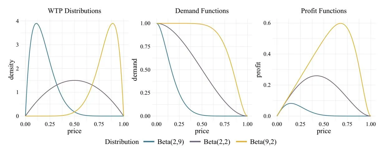
6.3. Valuation (WTP) Distributions: Right Skewed, Left Skewed, and Symmetric

To evaluate the performance of various MAB policies, it is crucial to consider different shapes of consumer valuation (WTP) distributions. Following Misra et al. (2019), we analyze three types of distributions using specific parameterizations of the Beta distribution: Beta(2, 9) for a right-skewed distribution, Beta(9, 2) for a left-skewed distribution, and Beta(2, 2) for a symmetric distribution. A graphical depiction of the willingness to pay, the demand curve, and the profit curve for each simulation setting is provided in Figure 3. A monopolist with perfect knowledge of the demand curve would set prices to maximize profit. The true optimal prices are 0.15 for Beta(2, 9), 0.42 for Beta(2, 2), and 0.68 for Beta(9, 2).

6.4. Algorithm Initialization

The algorithms are initialized with either a prior or by limited experimentation. For UCB, we assume a prior that encourages exploration by treating every untested price as if it has been tested once and resulted in a purchase.27 In contrast, TS and GP variants can use uninformed priors, enabling price selection even without prior data. To make the comparison more consistent,28 we have GP variants select the first price randomly, after which the price can be chosen using the dataestimated GP.

6.5. Results

Our results present several variants within the two main classes of algorithms (TS and UCB). Figure 4 illustrates the cumulative performance of each algorithm over time (or number of consumers), whereas Table 3 provides the exact values from Figure 4 at 500 and 2,500 consumers. Table 4 shows the uplift or gains from incorporating the two informational externalities relative to the baseline algorithms. Finally, Figure 5 presents a histogram of prices played, offering insight into the behavior of the different algorithms.

Figure 4. (Color online) Cumulative Percentages of Optimal Rewards (Profits)

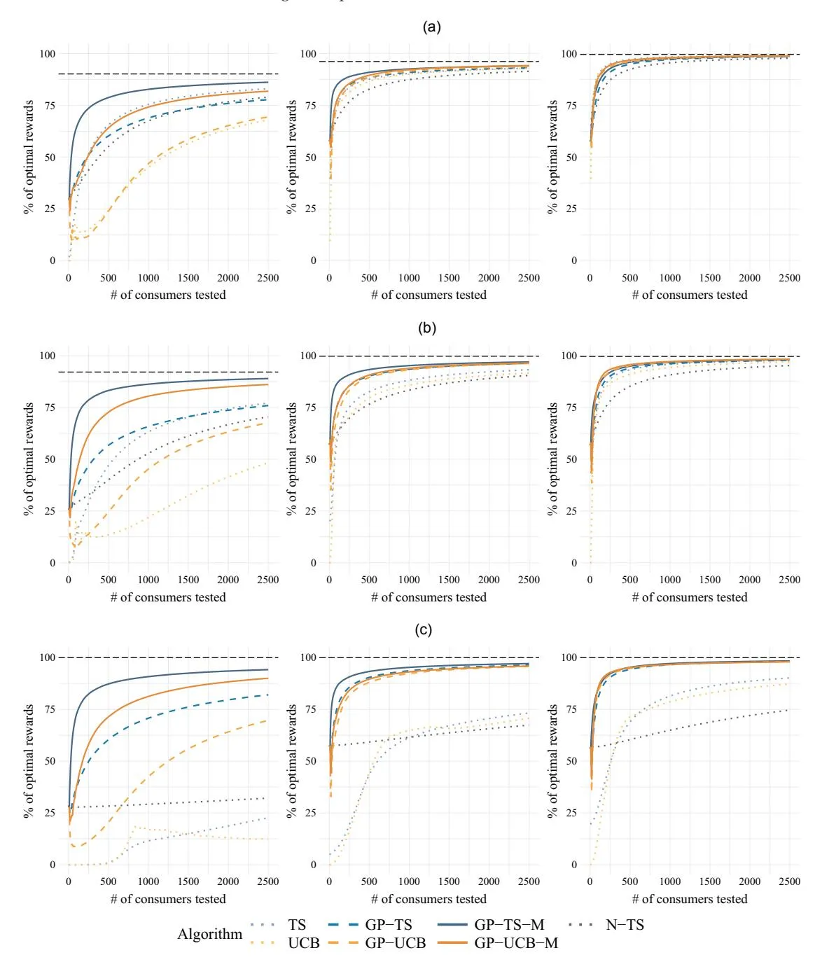
Notes. The lines represent the means of the cumulative expected percentages of optimal rewards across 1,000 simulations. The black horizontal lines represent the maximum obtainable reward given the price set, whereas 100% represents the true optimal reward given the underlying distribution. (a) Five arms: (a, i) right skewed: Beta(2, 9), (a, ii) symmetric: Beta(2, 2), and (a, iii) left skewed: Beta(9, 2). (b) Ten arms: (b, i) right skewed: Beta(2, 9), (b, ii) symmetric: Beta(2, 2), and (b, iii) left skewed: Beta(9, 2). (c) One hundred arms: (c, i) right skewed: Beta(2, 9), (c, ii) symmetric: Beta(2, 2), and (c, iii) left skewed: Beta(9, 2).

Table 3. Cumulative Percentages of Optimal Rewards (Profits)

	Percentage of price set maximum reward				Percentage of true optimal reward
Algorithm	B(2, 9)	B(2, 2)	B(9, 2)	Mean	B(2, 9)	B(2, 2)	B(9, 2)	Mean
				Panel A: After 500 consumers
5 arms
TS	72.7	91.2	97.6	87.2	65.6	87.7	97.2	83.5
GP-TS	66.8	92.0	95.3	84.7	60.2	88.4	94.9	81.2
GP-TS-M	87.3	94.6	96.3	92.7	78.7	90.9	95.9	88.5
N-TS	61.1	86.1	92.8	80.0	55.1	82.8	92.4	76.8
UCB	27.0	90.0	96.5	71.1	24.3	86.5	96.1	69.0
GP-UCB	26.5	92.0	96.6	71.7	23.9	88.5	96.2	69.5
GP-UCB-M	71.1	93.1	97.2	87.1	64.1	89.5	96.8	83.5
10 arms
TS	51.0	82.8	93.6	75.8	46.9	82.5	93.2	74.2
GP-TS	61.5	90.4	94.3	82.1	56.6	90.1	93.9	80.2
GP-TS-M	90.3	93.5	95.3	93.1	83.1	93.3	94.9	90.4
N-TS	43.5	76.8	85.6	68.6	40.0	76.5	85.2	67.3
UCB	14.6	79.8	91.4	61.9	13.5	79.6	91.0	61.3
GP-UCB	26.6	89.7	95.6	70.6	24.5	89.4	95.2	69.7
GP-UCB-M	78.9	90.9	96.0	88.6	72.7	90.6	95.6	86.3
100 arms
TS	1.0	43.4	69.0	37.8	1.0	43.4	69.0	37.8
GP-TS	60.4	90.5	94.4	81.8	60.4	90.5	94.4	81.8
GP-TS-M	87.3	93.3	95.4	92.0	87.3	93.3	95.4	92.0
N-TS	28.3	59.3	60.4	49.3	28.3	59.2	60.4	49.3
UCB	0.7	44.7	71.5	39.0	0.7	44.7	71.5	39.0
GP-UCB	20.6	88.1	94.8	67.8	20.6	88.1	94.8	67.8
GP-UCB-M	71.4	89.6	95.2	85.4	71.4	89.6	95.2	85.4
				Panel B: After 2,500 consumers
5 arms
TS	92.1	96.6	99.4	96.1	83.0	92.9	99.0	91.7
GP-TS	86.3	96.8	98.9	94.0	77.8	93.1	98.5	89.8
GP-TS-M	95.5	97.8	99.1	97.5	86.1	94.1	98.7	93.0
N-TS	87.6	95.1	98.2	93.6	79.0	91.4	97.7	89.4
UCB	75.4	96.6	99.1	90.4	67.9	92.9	98.7	86.5
GP-UCB	77.0	97.5	99.2	91.2	69.4	93.8	98.8	87.3
GP-UCB-M	90.8	98.0	99.3	96.0	81.8	94.2	98.9	91.6
10 arms
TS	83.7	93.5	98.1	91.8	77.1	93.2	97.7	89.3
GP-TS	82.4	96.6	98.2	92.4	75.9	96.3	97.7	90.0
GP-TS-M	96.6	97.2	98.4	97.4	88.9	96.9	98.0	94.6
N-TS	76.5	90.7	95.6	87.6	70.4	90.4	95.2	85.3
UCB	52.4	91.9	97.3	80.5	48.3	91.6	96.9	78.9
GP-UCB GP-UCB-M	73.4 93.5	96.5 96.8	98.6 98.7	89.5 96.3	67.6 86.0	96.2 96.5	98.2 98.3	87.3 93.6
100 arms TS	22.7	73.3	90.2	62.1	22.7	73.3	90.2	62.1
GP-TS	82.0	96.4	98.2	92.2	82.0	96.4	98.2	92.2
GP-TS-M	94.2	97.1	98.4	96.6	94.2	97.1	98.4	96.6
N-TS	32.2	67.4	74.7	58.1	32.2	67.4	74.7	58.1
UCB	12.3	70.8	87.2	56.8	12.3	70.8	87.2	56.8
GP-UCB	69.7	95.8	98.1	87.9	69.7	95.8	98.1	87.8
GP-UCB-M	90.0	95.9	98.0	94.7	90.0	95.9	98.0	94.7

Notes. The table provides mean cumulative percentage of optimal rewards (averaged across independent 1,000 simulations) after 500 and 2,500 consumers. The bolded values denote the unweighted means across the three conditions.

6.5.1. Main Results: Cumulative Performance. The performances of the algorithms are shown in Figure 4, which reports the cumulative percentage of optimal rewards relative to the case when the optimal arm (price) is played.29 In Figure 4, the horizontal black dashed lines represent the maximum obtainable rewards given the price set (i.e., the ratio of the reward obtained from playing the best price within the price set to the

Table 4. Uplifts in Performance from Informational Externalities

	WTP	TS			UCB
Uplifts	distribution	5 arms	10 arms	100 arms	5 arms	10 arms	100 arms
Panel A: After 500 consumers
Uplift from 1st externality	B(2, 9)	-7.9%	21.6%	6,011%	1.8%	89.7%	2,793%
(incorporating continuity		(-8.6 to -7.2)	(20.2 to 23.1)	(5,905 to 6,118)	(-0.4 to 4.0)	(84.2 to 95.2)	(2,723 to 2,864)
via GPs)	B(2, 2)	0.9%	9.4%	108%	2.3%	12.5%	96.9%
	D(0.5)	(0.6 to 1.3)	(8.9 to 9.9)	(108 to 109)	(1.9 to 2.8)	(12.0 to 13.0)	(96.3 to 97.6)
	B(9, 2)	-2.4%	0.8%	36.9%	0.1%	4.6%	32.7%
	M	(-2.6 to -2.1)	(0.6 to 1.0)	(36.5 to 37.2)	(0.0 to 0.3)	(4.4 to 4.8)	(32.5 to 32.8) 74.0%
	Mean	-2.7% (-3.0 to -2.5)	8.2% (7.8 to 8.5)	116% (116 to 117)	0.9% (0.6 to 1.2)	13.7% (13.2 to 14.1)	74.0% (73.5 to 74.6)
Uplift from 2nd externality	B(2, 9)	31.4%	48.6%	46.2%	177%	238%	291%
(incorporating monotonicity)	D(0, 0)	(30.3 to 32.5)	(47.0 to 50.2)	(44.5 to 47.9)	(171 to 182)	(223 to 252)	(277 to 306)
	B(2, 2)	2.9%	3.6%	3.2%	1.3%	1.4%	1.9%
	B(0, 2)	(2.6 to 3.2) 1.0%	(3.1 to 4.0)	(2.8 to 3.7)	(0.9 to 1.6)	(1.0 to 1.9)	(1.4 to 2.3)
	B(9, 2)	(0.8 to 1.3)	1.1% (0.9 to 1.3)	1.1% (0.9 to 1.2)	0.6% (0.5 to 0.7)	0.5% (0.4 to 0.6)	0.4% (0.3 to 0.6)
	Mean	9.1%	12.8%	12.6%	20.1%	24.0%	(0.3 to 0.6) 26.1 %
	1416011	(8.8 to 9.4)	(12.5 to 13.2)	(12.2 to 13.0)		(23.5 to 24.5)	(25.7 to 26.6)
TI 1:6.6. 1 d 1:0:	B(2, 0)
Uplift from both externalities	B(2, 9)	20.4%	78.5%	8,727%	174%	466%	9,955%
	B(2, 2)	(19.5 to 21.4) 3.8%	(76.9 to 80.1) 13.2%	(8,585 to 8,869) 115%	(168 to 180) 3.6%	(456 to 477) 14.0%	(9,904 to 10,006) 100%
	B(2, 2)	(3.4 to 4.2)	(12.7 to 13.7)	(114 to 116)	(3.1 to 4.0)	(13.5 to 14.5)	(99.7 to 101)
	B(9, 2)	-1.4%	1.9%	38.3%	0.8%	5.1%	33.2%
	D(>, L)	(-1.6 to -1.1)	(1.6 to 2.1)	(38.0 to 38.7)	(0.6 to 0.9)	(4.9 to 5.3)	(33.0 to 33.4)
	Mean	6.1%	21.9%	143%	21.1%	40.8%	119%
		(5.8 to 6.3)	(21.6 to 22.3)	(143 to 144)		(40.4 to 41.2)	(119 to 120)
		Panel B	: After 2,500 co	nsumers
Uplift from 1st externality	B(2, 9)	-6.3%	-1.5%	263%	2.2%	40.4%	465%
(incorporating continuity	,	(-6.5 to -6.1)	(-1.8 to -1.2)	(260 to 264)	(2.0 to 2.5)	(39.6 to 41.1)	(463 to 468)
via GPs)	B(2, 2)	0.2%	3.3%	31.6%	1.0%	5.0%	35.4%
		(0.0 to 0.4)	(3.1 to 3.6)	(31.3 to 31.8)	(0.8 to 1.2)	(4.8 to 5.2)	(35.2 to 35.7)
	B(9, 2)	-0.5%	0.0%	8.8%	0.1%	1.3%	12.5%
		(-0.6 to -0.5)	(-0.1 to 0.2)	(8.7 to 8.9)	(0.0 to 0.2)	(1.2 to 1.4)	(12.3 to 12.6)
	Mean	-2.0%	0.7%	48.5%	1.0%	10.6%	54.8%
		(-2.2 to -1.9)	(0.6 to 0.9)	(48.3 to 48.8)	(0.8 to 1.1)	(10.5 to 10.8)	(54.5 to 55.0)
Uplift from 2nd externality	B(2, 9)	10.8%	17.3%	14.9%	17.9%	27.6%	29.4%
(incorporating monotonicity)		(10.5 to 11.1)	(16.9 to 17.7)	(14.6 to 15.3)	(17.4 to 18.4)	(27.0 to 28.1)	(28.9 to 30.0)
-	B(2, 2)	1.1%	0.7%	0.8%	0.4%	0.3%	0.2%
		(0.9 to 1.2)	(0.5 to 0.9)	(0.6 to 1.0)	(0.3 to 0.6)	(0.1 to 0.5)	(0.0 to 0.3)
	B(9, 2)	0.2%	0.3%	0.3%	0.1%	0.1%	-0.1%
		(0.1 to 0.3)	(0.2 to 0.4)	(0.2 to 0.3)	(0.1 to 0.2)	(0.1 to 0.2)	(-0.2 to 0.0)
	Mean	3.5%	5.2%	4.8%	4.9%	7.2%	7.8%
		(3.4 to 3.7)	(5.0 to 5.3)	(4.6 to 4.9)	(4.8 to 5.1)	(7.1 to 7.4)	(7.6 to 7.9)
Uplift from both externalities	B(2, 9)	3.8%	15.4%	316%	20.5%	78.8%	631%
		(3.5 to 4.0)	(15.2 to 15.7)	(314 to 319)	(20.0 to 21.0)	(78.0 to 79.7)	(628 to 634)
	B(2, 2)	1.3%	4.0%	32.6%	1.4%	5.3%	35.6%
	D(C 2)	(1.1 to 1.5)	(3.8 to 4.3)	(32.3 to 32.9)	(1.3 to 1.6)	(5.1 to 5.5)	(35.4 to 35.9)
	B(9, 2)	-0.3%	0.3%	9.1%	0.2%	1.5%	12.4%
	Maan	(-0.4 to -0.3)	(0.2 to 0.4)	(8.9 to 9.2)	(0.2 to 0.3)	(1.4 to 1.6)	(12.2 to 12.5)
	Mean	1.4%	5.9% (5.8 to 6.1)	55.6%	6.0%	18.6%	66.7%
		(1.3 to 1.6)	(5.8 to 6.1)	(55.4 to 55.8)	(5.8 to 6.1)	(18.4 to 18.8)	(66.5 to 67.0)

Notes. The table provides mean uplifts (averaged across 1,000 independent simulations) along with their corresponding 99% confidence intervals calculated using a paired t-test. The bolded values denote the weighted means across the three conditions.

true optimal reward). The value of this line increases as the price set enlarges, approaching the true optimal of 100%. Visually, algorithms with no informational externalities are represented with dots in Figure 4, those with

the first informational externality (i.e., the GP) are represented with dashes in Figure 4, and those with both informational externalities are represented with solid lines in Figure 4. UCB variants are shown in warm

Figure 5. (Color online) Histogram of Prices Played

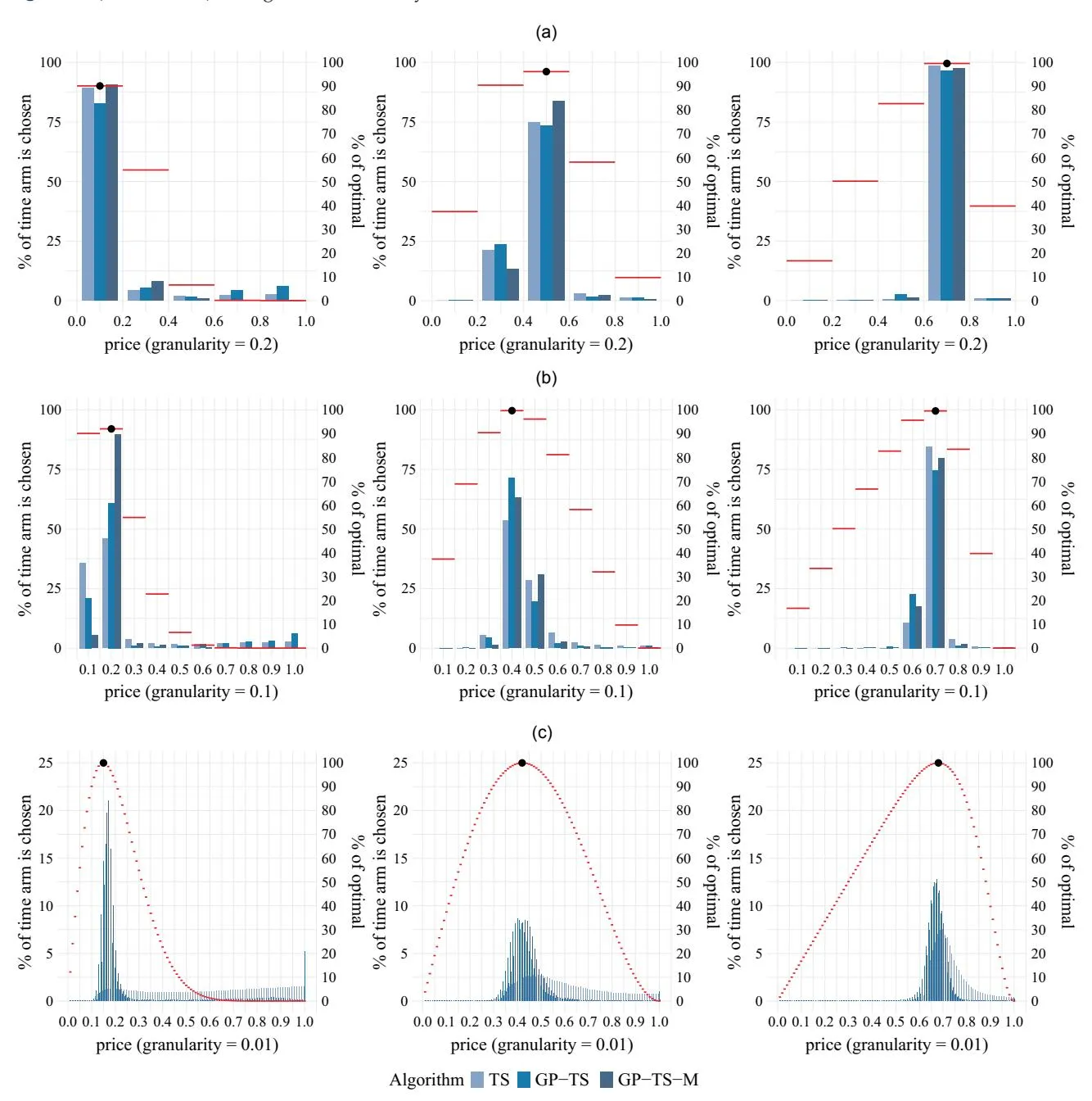
Notes. Each subfigure has two y axes, with price as the common x axis. The left y axis corresponds to the bar plots and represents the percentage of time that each arm is chosen (based on 2,500 consumers and averaged over 1,000 simulations). The right y axis corresponds to the red horizontal lines, which indicate the percentage of the true optimal reward obtainable at each corresponding price. The black dots mark the price that is optimal within the price set. (a) Five arms: (a, i) right skewed: Beta(2, 9), (a, ii) symmetric: Beta(2, 2), and (a, iii) left skewed: Beta(9, 2). (b) Ten arms: (b, i) right skewed: Beta(2, 9), (b, ii) symmetric: Beta(2, 2), and (b, iii) left skewed: Beta(9, 2). (c) One hundred arms: (c, i) right skewed: Beta(2, 9), (c, ii) symmetric: Beta(2, 2), and (c, iii) left skewed: Beta(9, 2).

(orange-based) colors, whereas TS variants are in cool (blue-based) colors in Figure 4.

In general, the results show that incorporating informational externalities improves algorithmic performance, although the effects vary across distributions and the number of arms. We explore this in more detail, starting with the case of five arms, illustrated in Figure 4(a). For the right-skewed Beta(2, 9) distribution, despite all algorithms eventually converging to the optimal price with sufficient learning, there is a significant separation in performance across algorithms even after 2,500 consumers. Incorporating the first informational externality—a Gaussian process—results in minimal improvement for UCB and a slight decrease in performance for TS. However, incorporating the second informational externality—monotonicity—leads to substantial performance gains for both GP-UCB and GP-TS. Finally, the N-TS algorithm performs similarly to GP-TS but is outperformed by GP-TS-M.

Next, we examine the symmetric and left-skewed distributions: Beta(2, 2) and Beta(9, 2), respectively. Although the ordering of algorithms’ performance is similar to the right-skewed Beta(2, 9) case, we observe that the differences between algorithms begin to shrink. This finding aligns with expectations outlined in Section 3 as the learning problem becomes easier when the optimal price is higher within the price set, allowing all algorithms to perform well. Averaging across all three distributions, the best-performing algorithm is GP-TS-M, achieving 92.7% of the maximum reward obtainable given the price set (and 88.5% of the true optimal) after 500 consumers and 97.5% of the maximum reward obtainable given the price set (93.0% of the true optimal) after 2,500 consumers (see Table 3).

We now increase the number of arms (prices). As the number of arms increases from 5 to 10, the rank ordering of the algorithms remains similar, with a few notable differences. In the Beta(2, 9) case, the first informational externality allows GP-TS to initially outperform TS, although TS narrowly surpasses it by 2,500 consumers. In contrast, GP-UCB now significantly outperforms UCB. Similarly, in both the Beta(2, 2) and Beta(9, 2) cases, the performance gap between GP-TS (GP-UCB) and TS (UCB) widens. Accordingly, the variation in performance across algorithms increases, with the lower-performing algorithms falling further behind the best-performing ones that use a GP. This growing difference occurs because of the first informational externality. Meanwhile, the second informational externality again provides a substantial gain in the Beta(2, 9) case but only minor improvements in the Beta(2, 2) and Beta(9, 2) cases. GP-TS-M continues to lead in performance, whereas N-TS performs comparably with TS and UCB.

When the number of arms increases from 10 to 100, the learning problem becomes more challenging, and the above patterns intensify. The gap between the best- and worst-performing algorithms widens further, driven primarily by the benefits of the first informational externality, which grows as the number of arms increases. Learning across 100 arms without leveraging nearby information requires significantly more data, making the advantages of shared learning through a Gaussian process increasingly pronounced. The second informational externality maintains similar effects regardless of the number of arms, reinforcing the substantial gain in the Beta(2, 9) case while providing only minor improvements in the Beta(2, 2) and Beta(9, 2) cases. GP-TS-M remains the best-performing algorithm, with N-TS still performing similarly to TS and UCB.

Having discussed the results across price granularities (number of arms), a question remains. In practice, a priori, how should a firm choose the price set? The general trade-off is that learning the optimal price is easier (more efficient) with fewer prices, but a higher optimum is possible when more prices are considered.

To illustrate, in the Beta(9, 2) case with five arms and after 2,500 consumers, GP-TS-M achieves 99.1% of the maximum reward possible given the chosen price set, which equates to 98.7% of the true optimal reward. Meanwhile, at the higher price granularity of 100 arms, GP-TS-M achieves 98.4% of both the maximum reward possible and the true optimal reward. In this case, the maximum reward possible with five arms happens to be close enough to the true optimal that the benefits of an easier learning problem outweigh the potential gains from being able to select a price closer to the true optimal. This is not always true. In the Beta(2, 9) case, the maximum reward possible is just 90.2% of the true optimal. As a result, despite GP-TS-M obtaining 95.5% of the maximum reward possible with 5 arms, it achieves just 86.1% of the true optimal—much worse than 100 arms, which achieves 94.2%. Thus, one important benefit of our proposed approach is that it makes it feasible to have a larger number of arms, enabling more precise discovery of the optimal price.

Overall, averaged across the three distributions, the highest-performing algorithm relative to the true optimal is GP-TS-M with 100 arms. Thus, we suggest that firms use many arms as this allows for higher potential gains that outweigh the losses from a more challenging learning problem, which are significantly mitigated by the incorporation of informational externalities.30 Additionally, GP-TS-M with 100 arms is also the bestperforming algorithm after 500 consumers, making this advice applicable for experiments of a wide range of reasonable durations.31

6.5.2. Uplifts: Performance Increase from Informational Externalities. We next examine the uplifts (the percentage improvement in cumulative profits from including an informational externality) in Table 4. This analysis quantitatively assesses the value of the externalities and clarifies how their impact depends on valuation distributions and the numbers of arms. Overall, we observe that although the uplift from the first externality is most influenced by the number of arms, the uplift from the second externality is primarily affected by the underlying WTP distribution.

After 2,500 consumers, the benefit of incorporating the first informational externality using GPs into both TS and UCB increases with the number of arms across all three distributions. Averaged across the distributions, the uplift for adding GP to TS is �2*:*0% for 5 arms, 0.7% for 10 arms, and 48.5% for 100 arms. For UCB, the corresponding uplifts are 1.0%, 10.6%, and 54.8%. For 100 arms, a common pattern for both TS and UCB emerges; the uplift sharply decreases as the optimal price increases, shifting from the right-skewed Beta(2, 9) to the left-skewed Beta(9, 2). These differences are substantial, with uplifts exceeding 200% for Beta(2, 9) but dropping to just 9%–13% for Beta(9, 2). This pattern persists for UCB across all numbers of arms, whereas for TS, the first externality actually decreases profits in the Beta(2, 9) case for both 5 and 10 arms.

For the second informational externality, the uplift patterns are consistent within the TS and UCB families of algorithms, specifically for GP-TS to GP-TS-M and GP-UCB to GP-UCB-M. Across the various numbers of arms, the uplifts remain stable, ranging from 3.5% to 5.2% for the TS family and from 4.9% to 7.8% for the UCB family. However, the uplifts vary substantially between distributions, with high gains concentrated in the Beta(2, 9) case; they drop to under 1% for Beta(2, 2) and approach 0% for Beta(9, 2).

For 500 consumers, the uplift patterns are similar to those discussed earlier but more pronounced. This is because comparative gains from algorithms often occur in the early rounds; over time, all algorithms eventually converge to the optimal price. This also implies that informational externalities are broadly valuable, regardless of whether the manager operates with a low experimentation budget (500 consumers) or a relatively high one (2,500 consumers).

6.5.3. Mechanism: Investigating the Prices Chosen by Algorithms. To understand why algorithms vary in performance, we examine the set of prices (arms) selected by each algorithm. Figure 5 presents three sets of three panels. Each graph in Figure 5 includes both left and right y axes. The left y axes in Figure 5 correspond to the blue bar plots, which show the percentage of time that each price was chosen. The right y axes in Figure 5 correspond to the red horizontal lines, which represent the proportion of optimal rewards obtainable by selecting that price. The highest red line in Figure 5 is further marked with a black dot, indicating the price that achieved the maximum reward within the price set as well as its percentage of the true optimal.

The value of the first informational externality (using a GP) increases with the number of arms, with the largest gains observed when there are 100 arms, whereas for 5 arms, the gains are negligible or even negative. This mechanism becomes clear when comparing Figure 5(a) (5 arms) with Figure 5(c) (100 arms). Because TS does not account for dependence across arms, it must learn the reward for each price individually, requiring extensive testing of each price. In contrast, GP-TS pools information across many low-performing arms, enabling it to focus on higher-reward areas more quickly without repeatedly testing each price. As the number of arms increases, these advantages become substantial.

However, with just five arms, TS can learn the reward distribution for each price relatively quickly and may even outperform GP-TS. For example, with five arms and a Beta(2, 9) distribution, GP-TS selects prices 0.7 and 0.9 (which provide minimal rewards) far more frequently than TS. When the arms or prices are far apart, the value of learning across arms can be negative. This is also exacerbated because the GP uses a single noise hyperparameter across all prices, leading to larger noise estimates in this price range. Consequently, the GP requires more learning to eliminate these prices from consideration than TS. Online Appendix EC.6 outlines a method to address this issue by incorporating heterogeneity in noise for GP modeling.

Meanwhile, for the second informational externality, the largest gains occurred in the Beta(2, 9) case, with positive uplifts diminishing as we move to the Beta(2, 2) and Beta(9, 2) cases. In panel (a, i) of Figure 5 (five arms, right skewed), all algorithms play the optimal price of 0.1 the majority of the time. However, both TS and GP-TS play prices 0.7 and 0.9 with a nonnegligible frequency, whereas GP-TS-M almost never selects these prices. Because these arms provide nearly zero reward, playing them is quite costly, which highlights the superior performance of GP-TS-M.

To understand why this occurs, recall that profit is demand scaled by price, meaning that even if demands are learned equally across prices, uncertainty bounds around profits are increasing with price. Algorithms that do not consider monotonicity (such as TS and GP-TS) must invest significant resources to determine whether high prices are suboptimal. As monotonicity requires each demand curve to be monotonically decreasing, it eliminates many possible demand curves that TS and GP-TS cannot disregard. Specifically, it can lead to gains by excluding from consideration demand curves that upward slope at high prices when the true optimal is a low price. Thus, with minimal data, monotonicity effectively reduces the need to explore highnoise, low-profit regions, thus demonstrating its value.

This advantage, however, applies primarily when the optimal price is low. Because lower prices have smaller reward bounds, other algorithms can also quickly dismiss low-profit, low-price arms; for example, panels (a, i), (b, i), and (c, i) of Figure 5 show that all of the algorithms rarely played prices below 0.5. Ultimately, the advantage from incorporating the second informational externality diminishes as the optimal price within the price set increases, although it remains positive across all simulations that we ran.

6.5.4. Robustness: Alternative WTP Distributions. We also conduct several analyses to assess the robustness of the method developed here. First, in Online Appendix EC.5.1, we test our method in an empirical setting using a demand curve estimated from field data. In this setting, the optimal price was low within the price set considered, and the results accordingly aligned with the Beta(2, 9) case for 5, 10, and 100 arms. This lends credence to our main analysis and demonstrates the practical value and applicability of the method.

Next, because the GP-based method requires continuity of the demand curve, we consider cases where the demand curve has discontinuities at known prices specifically, left-digit bias (Thomas and Morwitz 2005), where consumers perceive a larger price increase when the left-digit changes (e.g., from $1.99 to $2.00 is perceived as greater than a one-cent increase). We find that even in this challenging situation, the informational externalities improve performance (see Online Appendix EC.5.2). However, if the left-digit bias is large enough, it may be more effective for a firm to use only the prices immediately preceding the discontinuities as the price set rather than adopting a finer price granularity.

Finally, to examine whether the proposed bandit algorithms provide a long-run or persistent advantage, we explore the case of time-varying (seasonal) demand in Online Appendix EC.5.3, where we introduce an unknown demand shock each period. Once again, we find that informational externalities, especially monotonicity, significantly enhance long-term profits. Notably, we find that learning is so efficient that when the shocks are large enough, GP-TS-M can achieve higher profits by restarting the bandit experiment at each shock rather than relying on prior data. For the other algorithms tested, however, the start-up cost outweighed the gains from more accurately learning the demand curve.

7. Conclusion and Future Research

We have proposed a method for efficient and robust learning of the relevant portion of the demand curve by using reinforcement learning in multiarmed bandits informed by microeconomic principles, specifically monotonicity of demand curves.

Notably, our algorithm outperformed baseline methods across a variety of scenarios, including number of arms and valuations distributions as well as challenging cases, like discontinuous and time-varying demand, and it achieved significant gains across both the shortand long-term horizons. Our method is particularly beneficial for managers with limited time for experimentation. By reducing the required experimentation time, our approach makes price experimentation more feasible, minimizing potential monetary losses and limiting negative consumer impact. Our method leverages informational externalities to enable testing a finer grid of prices, allowing firms to evaluate prices closer to the true optimal. This not only increases gains during the experiment but can also lead to long-term profit improvements when a near-optimal price is adopted after the experiment concludes.

There are several avenues to extend this research. First, the method could be adapted to settings involving multiple units purchased or multiple products, where consumer choices for one product inform the valuation distribution of related products. Second, applying the method to competitive environments, where competitors are experimenting with price levels and demand responses, would be valuable. More broadly, efficiently learning unknown demand curves with minimal experimental impact remains a significant challenge across many markets. This research contributes to addressing this challenge by closely integrating theory with algorithm development for effective learning.

Endnotes

• ¹ It is noteworthy that pricing differs from advertising, where companies are generally more willing to experiment (Simester et al. 2009, Sahni and Nair 2020, Goli et al. 2025).
• ² A separate line of work incorporates inventory constraints into pricing models (Chen et al. 2019, Miao and Wang 2024). These studies often introduce constraints on revenue or utilize exploration phases that involve significant price fluctuations, which may not be feasible in practice. Further, their solutions are typically driven by the characterization of the optimal posted price, differing from our approach.
• ³ The population of consumers has a population-level distribution of WTP, which corresponds directly to the demand curve.
• ⁴ This excludes dynamic situations where consumers may change over time or where current decisions are heavily influenced by future expectations. Such cases include strategic consumers (Nair 2007), learning (Erdem and Keane 1996, Yu et al. 2016), and stockpiling (Hendel and Nevo 2006, Ching and Osborne 2020). These assumptions are often implicit in field experiments, such as in the advertising literature (Hoban and Bucklin 2015, Lambrecht et al. 2018, Gordon et al. 2019). For instance, if strategic consumers believe that a firm offering discounts is experimenting and may discount further later, the observed treatment effect may not accurately reflect reality.
• ⁵ This assumption can be relaxed; the results will hold as long as the algorithm is deployed in a stable environment where (1) competitors do not change prices strategically in response to real-time changes and (2) firms are unconcerned with potential future competitors (Rubel 2013).
• ⁶ Inventory constraints are relevant when stock is limited, such as in clothing. When products are constrained, it may be preferable to forgo selling to one consumer to sell to another with a higher WTP.

For products without production constraints, such as a Netflix subscription, this issue does not arise.

• ⁷ Small differences are discussed in Online Appendix EC.6.

• ⁸ With unscaled prices {pe¹ ,: : :, pf*^A* }, the set of scaled prices can be created by dividing any price by the largest price in the set (i.e., pa � pe*^a =pf^A* ).

• ⁹ Simply, the reward obtained from a potential consumer who purchases is the price charged minus the cost.

• ¹⁰ Formulating the bandit problem as a statistical problem (regret) rather than an optimization problem (maximizing cumulative reward) lends itself better to theoretical guarantees (Cohen and Treetanthiploet 2020).

• ¹¹ Theoretical guarantees often state that an algorithm has the lowest possible bound for expected regret; however, this is subtly different from empirical performance, which may be higher for algorithms without such theoretical properties. For example, it is proven that under certain conditions, UCB has the lowest possible bound for expected regret (Auer et al. 2002). However, empirically, under the same conditions, it is often outperformed by greedy algorithms with respect to maximizing rewards (Bayati et al. 2020).

• ¹² Among a set of algorithms, the one with the lowest cumulative regret is the same as the one with the highest cumulative rewards.

• ¹³ If the exploration term were zero, this would be equivalent to a fully greedy algorithm.

• ¹⁴ An alternative approach would be to use a parametric model, such as combining generalized linear models with UCB (Filippi et al. 2010), and restrict the coefficients to obtain weakly decreasing demand functions.

• ¹⁵ This is also incorporated to some degree in the UCB algorithm, which models both a term for the sample mean of each arm and an exploration bonus dependent on the bounds surrounding those sample means.

• ¹⁶ This approach can be thought of as a greedy-based GP algorithm. This was tested in Srinivas et al. (2009, p. 4), who found that it was “too greedy too soon and tends to get stuck in shallow local optima,” leading the algorithm to underexplore and produce inaccurate results.

• ¹⁷ In our setup, we use only the prices from the test set, although it is possible to estimate for any arbitrary price.

• ¹⁸ Intuitively, this can be thought of as the length of the “wiggles.”

• ¹⁹ Bayesian tuning methods are often too slow and not suitable for real-time bandit settings.

• ²⁰ For example, consider two close input points (x axis) that have very different outputs (y axis). One possible explanation is that the data are accurate, and the GP requires shape parameters that permit sufficiently high variation to capture large output differences from nearby inputs. Alternatively, the true outputs may be close together, but the data are very noisy; in this case, the previous shape parameters would be overfitting.

• ²¹ As we use purchase rates rather than purchase decisions as the training data, we also need to divide by nat at each price. See Online Appendix EC.2 for details.

• ²² Another possible initialization method is to set arbitrary hyperparameters and model the GP without data. Both methods are practical, with only minor differences in overall performance (under 1% in all our simulations), and neither method consistently outperforms the other.

• ²³ D^∗ is a random variable denoting the Gaussian process posterior prediction.

• ²⁴ Srinivas et al. (2009) found in their experiments that δ � 0*:*1 works well empirically, and we use that value here. Other values of β may

• perform better in different simulations, although determining β without past data is generally challenging (Brochu et al. 2010).

• ²⁵ We make a slight adjustment by relaxing the monotonicity assumption, requiring monotonicity only at the knot points rather than across all points.

• ²⁶ Although prices could be updated every period (i.e., for each consumer), this may be impractical in real-world settings. To better reflect industry practices, we change prices every 10 consumers as in Misra et al. (2019).

• ²⁷ An alternative approach is to test each price before applying the UCB policy; however, our initialization priors allow for the possibility of not testing every price, which can improve algorithmic performance.

• ²⁸ When faced with an uninformed prior, there are slight differences in the distribution of the first price chosen by the monotonic and nonmonotonic algorithms. This can lead to minute differences in performance (under 1% and usually around 0%) depending on the underlying WTP distribution attributable solely to the first price decision, which we mitigate by choosing the first price randomly.

• ²⁹ There are two sources of variation between simulations: one from the algorithm itself and another from the exact WTP draws from the true distribution. Using expected rewards from playing a price reduces the variation caused by WTP draws, allowing for a cleaner comparison of algorithmic performance. Misra et al. (2019) also use expected rewards in their analysis.

• ³⁰ Across the three distributions that we tested, with 100 arms, the maximum reward obtainable was at least 99.99% of the true optimal, suggesting that 100 arms may be sufficient. Further testing on a wider variety of WTP distributions would be useful.

• ³¹ If the experiment becomes sufficiently short, there will eventually be a point where a smaller price set will perform better.

References

• Aghion P, Bolton P, Harris C, Jullien B (1991) Optimal learning by experimentation. Rev. Econom. Stud. 58(4):621–654.

• Agrawal R (1995) Sample mean based index policies by O(log n) regret for the multi-armed bandit problem. Adv. Appl. Probab. 27(4):1054–1078.

• Agrawal S, Goyal N (2012) Analysis of Thompson sampling for the multi-armed bandit problem. Mannor S, Srebro N, Williamson RC, eds. Proc. 25th Annual Conf. Learn. Theory, vol. 23 (PMLR, New York), 39.1–39.26.

• Aparicio D, Simester D (2022) Price frictions and the success of new products. Marketing Sci. 41(6):1057–1073.

• Auer P (2002) Using confidence bounds for exploitation-exploration trade-offs. J. Machine Learn. Res. 3(November):397–422.

• Auer P, Cesa-Bianchi N, Fischer P (2002) Finite-time analysis of the multiarmed bandit problem. Machine Learn. 47(2–3):235–256.

• Bayati M, Hamidi N, Johari R, Khosravi K (2020) Unreasonable effectiveness of greedy algorithms in multi-armed bandit with many arms. Larochelle H, Ranzato M, Hadsell R, Balcan MF, Lin H, eds. Adv. Neural Inform. Processing Systems, vol. 33 (Curran Associates Inc., Red Hook, NY), 1713–1723.

• Bergemann D, Schlag KH (2008) Pricing without priors. J. Eur. Econom. Assoc. 6(2–3):560–569.

• Besbes O, Zeevi A (2009) Dynamic pricing without knowing the demand function: Risk bounds and near-optimal algorithms. Oper. Res. 57(6):1407–1420.

• Botev Z, Belzile L (2025) TruncatedNormal: Truncated multivariate normal and student distributions. https://github.com/lbelzile/ truncatednormal.

• Brochu E, Hoffman MW, de Freitas N (2010) Portfolio allocation for Bayesian optimization. Preprint, submitted September 28, https:// arxiv.org/abs/1009.5419.

• Chapelle O, Li L (2011) An empirical evaluation of Thompson sampling. Shawe-Taylor J, Zemel R, Bartlett P, Pereira F, Weinberger KQ, eds. Adv. Neural Inform. Processing Systems, vol. 24 (Curran Associates Inc., Red Hook, NY), 2249–2257.

• Chatterjee S, Sen S (2021) Regret minimization in isotonic, heavytailed contextual bandits via adaptive confidence bands. Preprint, submitted October 19, https://arxiv.org/abs/2110.10245.

• Chen Q, Jasin S, Duenyas I (2019) Nonparametric self-adjusting control for joint learning and optimization of multiproduct pricing with finite resource capacity. Math. Oper. Res. 44(2): 601–631.

• Cheshire J, Me´nard P, Carpentier A (2020) The influence of shape constraints on the thresholding bandit problem. Abernethy J, Agarwal S, eds. Proc. Thirty Third Conf. Learn. Theory, vol. 125 (PMLR, New York), 1228–1275.

• Ching AT, Osborne M (2020) Identification and estimation of forwardlooking behavior: The case of consumer stockpiling. Marketing Sci. 39(4):707–726.

• Chowdhury SR, Gopalan A (2017) On kernelized multi-armed bandits. Precup D, Teh YW, eds. Proc. 34th Internat. Conf. Machine Learn., vol. 70 (PMLR, New York), 844–853.

• Cohen SN, Treetanthiploet T (2020) Asymptotic randomised control with applications to bandits. Preprint, submitted October 14, https://arxiv.org/abs/2010.07252.

• Dann C, Mansour Y, Mohri M, Sekhari A, Sridharan K (2022) Guarantees for epsilon-greedy reinforcement learning with function approximation. Chaudhuri K, Jegelka S, Song L, Szepesvari C, Niu G, Sabato S, eds. Proc. 39th Internat. Conf. Machine Learn., vol. 162 (PMLR, New York), 4666–4689.

• Dholakia U (2015) The risks of changing your prices too often. Harvard Bus. Rev. (July 6), https://hbr.org/2015/07/the-risks-of-changingyour-prices-too-often?ab=HP-hero-for-you-text-2.

• Duvenaud D (2014) Automatic model construction with Gaussian processes. PhD thesis, University of Cambridge, Cambridge, UK.

• Erdem T, Keane MP (1996) Decision-making under uncertainty: Capturing dynamic brand choice processes in turbulent consumer goods markets. Marketing Sci. 15(1):1–20.

• Ferreira KJ, Simchi-Levi D, Wang H (2018) Online network revenue management using Thompson sampling. Oper. Res. 66(6):1586–1602.

• Filippi S, Cappe O, Garivier A, Szepesva´ri C (2010) Parametric bandits: The generalized linear case. Lafferty J, Williams C, Shawe-Taylor J, Zemel R, Culotta A, eds. Adv. Neural Inform. Processing Systems, vol. 23 (Curran Associates Inc., Red Hook, NY).

• Furman J, Simcoe T (2015) The economics of big data and differential pricing. The White House President Barack Obama (blog) (February 6), https://obamawhitehouse.archives.gov/blog/2015/02/06/ economics-big-data-and-differential-pricing.

• Gittins J (1974) A dynamic allocation index for the sequential design of experiments. Gittins JC, Jones DM, eds. Progress in Statistics (North-Holland, Amsterdam), 241–266.

• Goli A, Reiley DH, Zhang H (2025) Personalizing ad load to optimize subscription and ad revenues: Product strategies constructed from experiments on pandora. Marketing Sci. 44(2):327–352.

• Gordon BR, Zettelmeyer F, Bhargava N, Chapsky D (2019) A comparison of approaches to advertising measurement: Evidence from big field experiments at Facebook. Marketing Sci. 38(2): 193–225.

• Guntuboyina A, Sen B (2018) Nonparametric shape-restricted regression. Statist. Sci. 33(4):568–594.

• Handel BR, Misra K (2015) Robust new product pricing. Marketing Sci. 34(6):864–881.

• Hanssens DM, Pauwels KH (2016) Demonstrating the value of marketing. J. Marketing 80(6):173–190.

• Hauser JR, Urban GL, Liberali G, Braun M (2009) Website morphing. Marketing Sci. 28(2):202–223.

• Hendel I, Nevo A (2006) Measuring the implications of sales and consumer inventory behavior. Econometrica 74(6):1637–1673.

• Hill DN, Nassif H, Liu Y, Iyer A, Vishwanathan S (2017) An efficient bandit algorithm for realtime multivariate optimization. Proc. 23rd ACM SIGKDD Internat. Conf. Knowledge Discovery Data Mining (Association for Computing Machinery, New York), 1813–1821.

• Hoban PR, Bucklin RE (2015) Effects of internet display advertising in the purchase funnel: Model-based insights from a randomized field experiment. J. Marketing Res. 52(3):375–393.

• Huang Y, Ellickson PB, Lovett MJ (2022) Learning to set prices. J. Marketing Res. 59(2):411–434.

• Jindal P, Zhu T, Chintagunta P, Dhar S (2020) Marketing-mix response across retail formats: The role of shopping trip types. J. Marketing 84(2):114–132.

• Kawale J, Bui HH, Kveton B, Tran-Thanh L, Chawla S (2015) Efficient Thompson sampling for online matrix-factorization recommendation. Cortes C, Lawrence N, Lee D, Sugiyama M, Garnett R, eds. Adv. Neural Inform. Processing Systems, vol. 28 (Curran Associates Inc., Red Hook, NY), 1297–1305.

• Kermisch R, Burns D (2018) Is pricing killing your profits? Bain & Company. Accessed June 16, 2018, http://www.bain.com/ publications/articles/is-pricing-killing-your-profits.aspx.

• Lai TL, Robbins H (1985) Asymptotically efficient adaptive allocation rules. Adv. Appl. Math. 6(1):4–22.

• Lambrecht A, Tucker C, Wiertz C (2018) Advertising to early trend propagators: Evidence from Twitter. Marketing Sci. 37(2):177–199.

• Maatouk H, Bay X (2017) Gaussian process emulators for computer experiments with inequality constraints. Math. Geosciences 49(5): 557–582.

• Miao S, Wang Y (2024) Demand balancing in primal-dual optimization for blind network revenue management. Preprint, submitted April 6, https://arxiv.org/abs/2404.04467.

• Micchelli CA, Xu Y, Zhang H (2006) Universal kernels. J. Machine Learn. Res. 7(12):2651–2667.

• Misra K, Schwartz EM, Abernethy J (2019) Dynamic online pricing with incomplete information using multiarmed bandit experiments. Marketing Sci. 38(2):226–252.

• Nair H (2007) Intertemporal price discrimination with forwardlooking consumers: Application to the US market for console video-games. Quant. Marketing Econom. 5(3):239–292.

• Oren SS, Smith SA, Wilson RB (1982) Nonlinear pricing in markets with interdependent demand. Marketing Sci. 1(3):287–313.

• Rao RC, Bass FM (1985) Competition, strategy, and price dynamics: A theoretical and empirical investigation. J. Marketing Res. 22(3): 283–296.

• Ringbeck D, Huchzermeier A (2019) Dynamic pricing and learning: An application of Gaussian process regression. Preprint, submitted June 24, http://dx.doi.org/10.2139/ssrn.3406293.

• Rothschild M (1974) A two-armed bandit theory of market pricing. J. Econom. Theory 9(2):185–202.

• Rubel O (2013) Stochastic competitive entries and dynamic pricing. Eur. J. Oper. Res. 231(2):381–392.

• Sahni NS, Nair HS (2020) Does advertising serve as a signal? Evidence from a field experiment in mobile search. Rev. Econom. Stud. 87(3):1529–1564.

• Schwartz EM, Bradlow ET, Fader PS (2017) Customer acquisition via display advertising using multi-armed bandit experiments. Marketing Sci. 36(4):500–522.

• Shahriari B, Swersky K, Wang Z, Adams RP, De Freitas N (2015) Taking the human out of the loop: A review of Bayesian optimization. Proc. IEEE 104(1):148–175.

• Simester D, Hu Y, Brynjolfsson E, Anderson ET (2009) Dynamics of retail advertising: Evidence from a field experiment. Econom. Inquiry 47(3):482–499.

• Srinivas N, Krause A, Kakade SM, Seeger M (2009) Gaussian process optimization in the bandit setting: No regret and experimental design. Preprint, submitted December 21, https://arxiv. org/abs/0912.3995.

• Thomas M, Morwitz V (2005) Penny wise and pound foolish: The left-digit effect in price cognition. J. Consumer Res. 32(1):54–64.

• Thompson WR (1933) On the likelihood that one unknown probability exceeds another in view of the evidence of two samples. Biometrika 25(3/4):285–294.

• Tirole J (1988) The Theory of Industrial Organization (MIT Press, Cambridge, MA).

• Urteaga I, Wiggins CH (2018) Nonparametric Gaussian mixture models for the multi-armed bandit. Preprint, submitted August 8, https://arxiv.org/abs/1808.02932.

• Wang Y, Chen B, Simchi-Levi D (2021) Multimodal dynamic pricing. Management Sci. 67(10):6136–6152.

• Williams CK, Rasmussen CE (2006) Gaussian Processes for Machine Learning, vol. 2 (MIT Press, Cambridge, MA).

• Yu M, Debo L, Kapuscinski R (2016) Strategic waiting for consumergenerated quality information: Dynamic pricing of new experience goods. Management Sci. 62(2):410–435.

• Zhang L, Chung DJ (2020) Price bargaining and competition in online platforms: An empirical analysis of the daily deal market. Marketing Sci. 39(4):687–706.

• Zhao H, He J, Zhou D, Zhang T, Gu Q (2023) Variance-dependent regret bounds for linear bandits and reinforcement learning: Adaptivity and computational efficiency. Neu G, Rosasco L, eds. Proc. Thirty Sixth Conf. Learn. Theory, vol. 195 (PMLR, New York), 4977–5020.