Optimal Budget Allocation Across Search Advertising Markets

One critical operational decision facing online advertisers when they engage in sponsored search advertising is concerned with the allocation of a limited advertising budget. In particular, dealing with multi-keyword search markets over multiple decision periods poses significant decision-making challenges. In this paper, we develop a novel budget allocation optimization model with multiple search advertising markets and a finite time horizon. One key element of our modeling work is developing a customized advertising response function when considering distinctive features of sponsored search, including the quality score and the dynamic advertising effort. We derive a feasible solution to our budget model and study its properties. Computational experiments are conducted on real-world data to evaluate our budget model and perform parameter sensitivity analysis. Experimental results indicate that our budget allocation strategy significantly outperforms several baseline strategies. In addition, the identified properties derived from the solution process illuminate critical managerial insights for advertisers in sponsored search.

Keywords: sponsored search; budget allocation; budget strategy; search markets History: Accepted by Alexander Tuzhilin, (former) Area Editor for Knowledge and Data Management; received September 2012; revised October 2013, July 2014; accepted September 2014.

1. Introduction

In recent years, sponsored search has evolved into one of the most prominent online advertising channels. Search advertisements have also become the primary revenue source for search engines. For example, Google gained 91% of its total revenue from sponsored search in 2013 (Google Inc. 2014). Because advertisers are spending increasing amounts of advertising budgets on search engines, there is an urgent need for analytical frameworks and tools that can help these advertisers maximize the effectiveness of their advertising budgets and survive fierce competition in the search advertising space.

From an operational standpoint, advertising budget allocation decisions are the first and foremost problem faced by advertisers when conducting sponsored search auctions. There are many challenges associated with budget allocation in sponsored search. First, advertisers usually do not have sufficient knowledge and time to make effective budget decisions in sponsored search because the underlying mechanism is quite complex and the bidding process is dynamic over time. Second, it is becoming increasingly difficult for an advertiser to deal with budget allocation decisions simultaneously across several search markets. Third, it is not always the case that spending more in advertising leads to higher profits.

Although the industry needs have been clear, the academic literature on search auction-specific advertising budget allocation has been sparse. This paper aims to help bridge this critical gap by formulating a fairly general optimization-based budget allocation model that can tackle multiple search markets simultaneously over a finite planning horizon. (Note that we use search engines and search markets interchangeably in the rest of this paper. That is, each search engine is a search market.) This model is dynamic in nature and can capture distinctive features of sponsored search advertising. First, we extend the advertising response function, given by Sethi (1983), to better suit the sponsored search advertising scenario by

incorporating the dynamic advertising effort and quality score. The advertising effort represents the effective part of the advertising expenditure and is time dependent. Because almost all search engines have adopted quality-based ranking and pricing mechanisms in recent years, the quality of the advertisements (measured by the quality score) has become an influential factor that affects budget decisions in a major way. We assume a much more general and timevarying relationship between the advertising budget and the advertising effort to more accurately characterize sponsored search advertising. We also assume heterogeneous advertising effort elasticity based on the observation that sponsored search advertising involves advertising with varying degrees of expertise, different advertising schedules, dynamic bids, and other factors.

Based on this model, we offer a solution framework to derive the optimal budget allocation strategy, and we analyze various theoretical properties of the solution. Some notable properties are as follows: (1) The observation in traditional advertising that the marginal return of increased advertising expenditure is never increasing (Sasieni 1971) holds in sponsored search advertising as well. (2) Under the optimal budget allocation solution, the advertising effort is positively proportional to the product of the change of the accumulated payoff in a market, the change of the market share, and the advertising effort elasticity. (3) There exists a saturation level of advertising expenditures termed the “producer equilibrium” where the marginal payoff drops to zero in cases where budget constraints are not imposed.

We conduct computational experiments based on real-world data to evaluate our solution, explore identified properties of the solution, and perform sensitivity analysis. Experimental results show that our budget strategy outperforms several baseline strategies. In addition, our solution process and the derived heuristic strategy illuminate critical managerial insights for advertisers in sponsored search. Managerially, our analysis points to some interesting findings with relevance to advertisers in sponsored search advertising: (1) There exists a producer equilibrium without consideration of budget constraints. (2) Advertisers with increasing advertising effort elasticity should invest more of their budget in the later stages, but those with decreasing advertising effort elasticity should invest more of their budget in the earlier stages. (3) The gross advertising return has a dominating effect on the optimal budget strategy when it is relatively small.

The remainder of this paper is organized as follows: §2 provides the literature review. Section 3 presents an advertising budget allocation model across search advertising markets. Section 4 discusses the properties of the optimal solution and presents a solution framework. We then present the experimental results and related managerial implications in §5. Section 6 discusses implementation issues of our model applied in practice. Finally, we conclude this research and discuss future research directions in §7.

2. Literature Review

In this section, we first survey the literature on advertising response. We then focus on the topic of optimal advertising budget allocation in general and budgeting decisions in the specific context of sponsored search.

2.1. Advertising Response

In early literature related to advertising, advertising response functions are formulated to capture the relationship between advertising spending and sales (Sasieni 1971, Rao and Rao 1983). The pioneering work of Vidale and Wolfe (Vidale and Wolfe 1957) proposed the concept of advertising effectiveness and advertising response dynamics, which leads to the Vidale-Wolfe model. This model implies concavity and the existence of advertising spending saturation (Little 1979). Another important concept is advertising goodwill introduced by Nerlove and Arrow (Nerlove and Arrow 1962), stating that the current aggregated advertising effectiveness can influence budget decisions later on. Subsequent research explored extending the basic Vidale-Wolfe model to more complicated situations such as competition among advertisers (Erickson 1992) and stochastic disturbance in the marketing environment (Sethi 1983).

In uncertain markets where the response function is not known, stochastic models of the advertising budget decision have been developed to help with budget allocation decisions (Holthausen and Assmus 1982, Du et al. 2007, Yang et al. 2013). Holthausen and Assmus (1982) presented a model for allocating the advertising budget to market segments when sales response to advertising is uncertain. In this line of work, an efficient frontier is defined over expected profits, and the advertiser chooses the optimal allocation based on her preference function. Du et al. (2007) considered the advertising budget decision with uncertain advertising response as a Markov decision process and developed a stochastic model with two-dimension state variables to solve it. Sethi (1973) examined the optimal advertising schedule problem, extending the dynamic version of the Vidale-Wolfe advertising model. In later work, he considered a variation of that problem in which the objective functions of the deterministic and the stochastic problem are identical (Sethi 1983). Sethi’s response function also captures the word-ofmouth effect. In the work of Naik et al. (1998), three

phenomena—repetition wearout, copy wearout, and advertising quality restoration—were explicitly considered to extend the Nerlove-Arrow model by introducing an ordinary differential equation of the advertising quality.

2.2. Optimal Control of Advertising Budget

Previous research on marketing budget decisions has shown that profit improvement from better allocation across products or regions is much higher than that from simply increasing the overall budget (Tull et al. 1986, Fischer et al. 2011). Because of the dynamic nature of advertising markets, various dynamic programming approaches have been developed to find optimal solutions for budget allocation problems either over multiple products (Fischer et al. 2011) or among generic and specialized Web portals (Fruchter and Dou 2005). Fruchter and Dou (2005) utilized dynamic programming techniques to derive the analytical solution to the optimal budget allocation problem. Their conclusions indicate that budget allocation strategies rely nonlinearly on the targeted audiences, average click-through rates, and adverting effectiveness of websites. Thus advertisers are advised to switch more budgets into specialized Web portals to maximize click volumes in the long term. However, the payoff in their model considers only direct advertising effects (such as clicks) while ignoring effects on market shares and advertising responses. Fischer et al. (2011) explored the marketing budget allocation problem for multiproduct, multicountry firms with various marketing activities. They focused on the adjustment of the budget level during next year’s planning cycle by assuming that the total marketing budget has already been set at the firm level and is kept constant over the planning horizon. Their research findings suggest that budgets should be allocated according to the size of the business, the effectiveness of the marketing activities, and the growth potential of the product.

We note that previous research on optimal advertising budgets (or expenditures) does not apply to sponsored search advertising because of this market’s distinctive features, such as the heavy use of the quality score and the dynamic nature of the advertising activities. In this work, we extend the response function as given in Sethi (1983) to better suit the setting of sponsored search advertising.

2.3. Budget Strategies in Sponsored Search Advertising

Most search advertisers, especially those from small and medium-sized enterprises, have some budget constraints (Search Engine Watch 2006, Abrams et al. 2007). How to effectively allocate the limited advertising budget is a critical operational-level issue. However, the literature review uncovered only a few studies relevant to budget allocation across search markets in sponsored search auctions. Some research has investigated how to place bids over a set of keywords to maximize the advertiser’s expected number of clicks under a given budget (Özlük and Cholette 2007, Feldman et al. 2007, Muthukrishnan et al. 2010). Results from Özlük and Cholette (2007) showed that price elasticities of the click-through rate and response functions are key factors for budget decisions, and advertisers can improve profits by investing in more keywords under a certain threshold. Feldman et al. (2007) studied how to spread a given budget across keywords to gain maximal revenues, and proposed a two-bid uniform bidding strategy that randomizes bid prices between two bid prices on all keywords in the campaign until the actual daily budget is exhausted. Muthukrishnan et al. (2010) explored the stochastic version of this problem. In actual sponsored search advertising, advertisers are not allowed to spread their budget across keywords directly.

Another stream of related research is bid optimization. By considering bid dynamics and rankings of advertisers, Zhang and Feng studied a cyclical bid adjustment model in a two-player competition (Zhang and Feng 2005, 2011), where an equilibrium bidding price for two advertisers can be obtained. They also adopted an empirical strategy of the Markov switching regression to examine the existence of such cyclical bidding strategies. Yao and Mela (2011) developed a dynamic structural model of keyword advertising to explore how the interactions between search users, advertisers, and the search engine affect consumer welfare and firm profits. In that model, they used a pure-strategy Markov perfect equilibrium to model the bidder’s decision of whether and how much to bid to maximize the discounted expected future profits. Amin et al. (2012) cast the bidding optimization with a budget constraint as a Markov decision process with censored observations and correspondingly employed a reinforcement learning algorithm. Similarly, Gummadi et al. (2011) formulated the bidding optimization as a discounted Markov decision process and provided approximate optimal bidding strategy over a large number of auctions.

The problem settings for bidding determination versus budget allocation are quite different because they deal with disparate topics. The former often studies bid determination and dynamic adjustments on specific keywords at the microlevel of advertising decisions in sponsored search. These studies focus more on the properties and solutions of the game where several risk-neutral advertisers compete for a limited number of positions. In each period, an advertiser’s bidding strategy depends on bid prices set by other advertisers and her own setting such as the valuation for a click. The latter (i.e., budget allocation)

usually centers on budget allocation across markets, over multiple campaigns, and among different promotional activities at the macrolevel of advertising decisions in sponsored search.

Bid determination and budget allocation also have something in common. On one hand, research outcomes on bidding strategies might provide useful insights for budget competition among several advertisers in sponsored search, which is not in the scope of this work. Our work concerns budget allocation across several search markets for an individual advertiser. On the other hand, under a certain condition, the bid determination for a single query can be viewed as a special type of budget decision. However, such a setting fails to capture several distinctive features in budget decisions, including the saturation level of the market, relationships between advertising spending and market sales, aggregate advertising effects, and temporal effects of advertising spending over a finite time horizon. These features are all included in our budget allocation model.

During the entire life cycle of sponsored search advertising, budget decisions occur at three levels: allocation across search markets; temporal distribution over a series of slots (e.g., days); and adjustment of the remaining budget (e.g., daily budgeting). In a previous work (Yang et al. 2012), we developed a hierarchical budget optimization framework (BOF), considering the entire life cycle of advertising campaigns in sponsored search advertising. The BOF could support a set of strategies across different levels of abstractions (e.g., system, campaign, and keyword). In this paper we examine the budget allocation problem across search advertising markets (e.g., at the market level of the BOF). This work develops an optimal model of budget allocation across several search markets over a finite planning horizon by taking the advertising response function to capture market dynamics. We also assume a different response function to provide a better fit for budget decision scenarios, taking into account several distinctive features in sponsored search.

3. Optimal Budget Allocation Across Search Markets

3.1. Problem Statement

An important decision an advertiser faces when advertising her products and services via sponsored search is how to allocate the search engine advertising budget across multiple search engines.¹ The main reason for advertisers considering more than one search engine is to reach different target audiences. In other words, advertisers often prefer to advertise on more than one search engine to reach a wider selection of consumers. In this study, we consider using two search engines.

There are typically two types of budget situations for an advertiser. One is that there exists a given (exogenous) total budget level for a certain period of time. In the second scenario, an advertiser can spend according to advertising performance and does not have a specific total budget constraint. We term the decision problems under these two cases as constrained budget allocation (CBA) and unconstrained budget allocation (UBA), respectively. In both cases, the advertiser seeks to optimize the total profit gained from advertising through sponsored search within a certain period of time (T ). Decisions need to be made dynamically between time 601 T 7.

The notation used in this paper is listed in Table 1.

3.2. Model Formulation

We consider an advertiser who plans to allocate her search engine advertising budget B across two search engines. Let i denote the index of search engines.

Search Demand. Let mⁱ 4t5 be the potential search demand for search engine i at time t. The search demand on a search engine is defined as the total number of clicks on advertisements generated from the keywords related to the advertiser.

Revenue. Let cⁱ 4t5 be the proportion of effective clicks among mⁱ 4t5 in market i at time t. Let vⁱ 4t5 denote the revenue generated from an effective click. Let ⁱ 4t5 denote this advertiser’s market share on market i at time t and bⁱ 4t5 denote the advertising budget allocated to market i at time t. Then for market i at time t, mⁱ 4t5cⁱ 4t5 represents the total number of effective clicks, Cⁱ 4t5 = vⁱ 4t5mⁱ 4t5cⁱ 4t5 represents the total revenue (gross advertising return), and Cⁱ 4t5ⁱ 4t5 denotes the advertiser’s revenue in market i at time t.

Table 1 List of Terms

Terms	Definition
B	The total advertising budget
i	The index of a search market
mi 4t5	The potential search demands in market i at time t
ci 4t5	The proportion of effective clicks in market i at time t
vi 4t5	The revenue generated from an effective click in market i at time t
ˆi 4t5	An advertiser’s market share on market i at time t
È4t5	The vector of market shares for the advertiser at time t
bi 4t5	The advertising budget allocated in market i at time t
Ci 4t5	The gross advertising return in market i at time t
ui 4t5	The advertising effort in market i at time t
	The response constant
”	The market share decay constant
i 4t5	The advertising effort elasticity in market i at time t
qi 4t5	The advertiser’s quality score in market i at time t
R4t5	The present value of the remaining advertising budget at time t

¹ According to Varian (2006), the likely market structure for a search engine advertising market will be one with a few large providers in a given country or language group.

The goal of budget allocation is to maximize the following objective function:

$\sum_{i} \int_{0}^{T} e^{-rt} (v_i(t)m_i(t)c_i(t)\theta_i(t) - b_i(t)) dt, \qquad (1)$

where e ⁻r t is the discount factor.

In Equation (1), bⁱ 4t5 can be further written as bi 4t1È4t55, where È4t5 represents the vector of market shares.

3.2.1. Response Function for Search Engine Advertising. Aggregate advertising models relate product sales to advertising spending for a market. The Vidale-Wolfe advertising model is one of the pioneering and earliest works in this direction (Vidale and Wolfe 1957). This model defines the basic process of how sales evolve over time in response to advertising spending and thus can be used to capture the dynamics of our search advertising environments. Sethi (1983) adopted a variation of the Vidale-Wolfe model that captures several desirable characteristics one would intuitively attribute to advertising response, and discussed in more detail next.

According to the aggregate advertising response model in Sethi (1983), the relationship between the market share () and the advertising effort (u) satisfies the following differential equation:

$\mathrm{d}\theta/\mathrm{d}t = \rho u \sqrt{1-\theta} - \delta\theta,$

where u denotes the advertising effort; is the response constant measuring the effectiveness of advertising, i.e., response to advertising that acts positively on the unsold portion of the market; and is the market share decay constant determining the rate at which customers are lost due to forgetting or possibly due to competitive factors that act negatively on the sold portion of the market.

The advertising effort u and the response constant are very general terms, capturing the effective part of the budget and advertising. This applies to a wide range of advertising settings including ours. The square-root term ^√ 1 − captures several desirable properties, e.g., market share has a concave response to advertising (decreasing returns), there is a saturation advertising level (Little 1979, Krishnamoorthy et al. 2010), and it also captures the word-of-mouth effect as noted by Sorger (1989). These properties are general observations among different advertising settings including ours. Therefore, we inherited this model to develop the response function used in our budget optimization model.

To better suit the sponsored search advertising scenario, we extend the advertising response function in Sethi (1983) by incorporating the dynamic advertising effort, the zero decay constant, and the quality score, which are discussed in more detail next.

Advertising Effort and Elasticity. The advertising effort represents the effective part of the advertising budget (or expenditure). Only this part can generate positive advertising effects. According to Little (1979), it is assumed that an exponential relationship exists between the budget b and advertising effort u. That is, u = b exists, where denotes the advertising effort elasticity, which is represented as the percentage change in the advertising effort to the change of one percent in the advertising expenditure, i.e., 4u/u5/4b/b5. It is usually fixed as a constant. For example, Erickson (1992) empirically estimated that = 0005. The constant assumption might be explained by the uniform advertising performance by professional advertising agencies in traditional advertisements.

However, in much more dynamic sponsored search markets, an advertiser can make changes in her advertising content and strategy at any time in an advertising campaign. In addition, sponsored search advertising has more flexibility, in terms of keyword selection, bid determination, budget allocation, and advertising schedules, which affects the effectiveness of the advertising budget. As such, the relationship between b and u is time varying in different search advertising markets: uⁱ 4t5 = bⁱ 4t54t5 .

Decay Term. Another difference in the response function is that we assume zero decay.

In the advertising response function for traditional advertising, the decay constant is used to capture the negative effect: loss due to forgetting or possibly due to competitive factors that act negatively on the sold portion of the market (Sethi 1983). In other words, the lagged response (or the carryover effect) over the time period between exposure to advertising (i.e., the realization of the cost) and purchase (i.e., the measure of the payoff generation) is negatively affected by many factors such as forgetting and competitions. At the aggregate level, the direct relationship between the rate of change in sales and the advertising carryover effect is often characterized by a differential equation (Sethi 1977). It needs a much larger state space to truly model the carryover effect at the individual level, considering various types of cognitive factors and the temporal dependency between activities.

The sales decay rate refers to the proportion of sales lost in each time when advertising is reduced to zero, which ranges from large values to almost zero (Vidale and Wolfe 1957). In the case of durable goods, the decay term can be considered to approximate the effect of product breakage and returns, which is usually assumed to be insignificant and is ignored (Sethi et al. 2008). One possible reason for zero decay in durable goods is that the product purchase cycle is much longer than the advertising cycle (e.g., purchase every five years but advertising once a

year). This phenomenon also applies to search advertising, which is often conducted continuously (daily if not hourly). In search advertising, the product purchase cycle is definitely much longer than the advertising cycle. Aravindakshan and Naik (2011) designed a delay differential equation to capture the role of delayed forgetting in a model of awareness formation. Their model well explains some small decay phenomena as observed in Sutherland (2009).

Different advertising media have different lag structures and effects (Berkowitz et al. 2001). Traditional advertising (e.g., TV ads) usually takes the volume of sales as the profit. For a potential customer, there is a certain period between seeing the advertisement and making the purchase. During this period, some negative factors (e.g., forgetting) might cause the loss of sales. In search advertising, it is common to use the number of clicks received to measure the profit, e.g., the pay-per-click (PPC) model widely adopted by sponsored search advertising. In our model, the realization of the cost (i.e., when the customer clicks) and the payoff generation (also when the customer clicks) happen at exactly the same time. In the current search engine marketing market, an advertiser does not pay (no cost incurred) when the advertisements are shown on the search results page (after a user made a search). Instead, she is only charged when the advertisement is clicked. Other than the short advertising cycle, the fact that the realization of the advertising cost and the payoff generation happen at exactly the same time also supports our zero decay assumption. The reason is that it becomes very unlikely for the advertising effect to drop to zero before profit generation because there is no time lag between advertising occurrence and profit generation.

Therefore, we argue that the decay constant is insignificant in sponsored search advertising. However, we have conducted simulations to study the effect of small decay constant on market share. Market share is continuously dependent on the parameter . Let 4t5 denote the market share with respect to a decay constant at time t, ceteris paribus. Table 2 describes the relative error (e.g., 4⁰ 4t5 − 4t55/⁰ 4t5) with two different decay constants, e.g., = 0001 and = 00001, respectively. As we can see, compared to the one with zero decay, the variation of market share is very small with a small . Our results indicate that a small decay over a short, finite time horizon has very limited impact on the market share.

Based on our deliberation, we adopt the zero decay in our model (i.e., d/d^{t =} u^√ 1 − ).

Quality Score. In addition to the advertising budget, an advertiser’s quality score q also has significant influence over her capacity to gain market shares. Specifically, a higher quality score entitles an advertiser to pay less for each click, so the same advertising budget can result in a higher market share. When there is a strong positive correlation between bid price and relevance (quality), the quality scoreadjusted ranking mechanism facilitates better matching between advertisements and queries and thus leads to higher expected revenues for search engines (Feng et al. 2007, Zhang and Feng 2011).

Different search engines have different formulas calculating the quality score, which are often closely guarded business secrets. According to Google AdWords, the quality score is calculated based on a number of factors, including the keyword’s past click-through rate (CTR), the display URL’s past CTR, the overall CTR of all the ads and keywords (in the advertiser’s account), the quality of the landing page, the relevance between the keyword and the ad, the relevance between the keyword and the query, geographic performance, etc.

Many factors influencing the quality score can be affected by various advertising decisions including budget decisions. For example, the former three factors (i.e., the keyword’s past CTR, the display URL’s past CTR, and the overall CTR of all the ads and keywords) usually depend on bid determination strategies that determine the likelihood that the ad is displayed on the search engine result page and matching options (e.g., the exact match might lead to more target audiences). The latter four factors are concerned with the quality of the ad, the keyword selected, and the target population. To some degree, the market-level total advertising budget also impacts the value range of these factors, which in turn affects the quality score. That is, the quality score is indirectly determined by budget decisions at the market level.

If we assume a functional form for the quality score (e.g., a linear function of budget), it will introduce bias because the calculation of the quality score is a closely guarded secret and is related to many factors. In the experiments, the quality score is not a fixed value. We use CTR obtained from real data as the quality score because CTR directly measures the effectiveness of an advertisement and is the core component for the

Table 2 The Relative Error with Different

”	t = 1	t = 2	t = 3	t = 4	t = 5	t = 6	t = 7	t = 8
” = 0001	0000503	0001001	0001493	0001979	0002460	0002935	0003405	0003868
” = 00001	0000050	0000100	0000150	0000200	0000249	0000298	0000347	0000395

quality score. This allows us to indirectly capture the endogeny of the quality score since CTR is affected by budget and many other decision variables.

Therefore, the advertising response function for search advertisements is given as follows:

$d\theta/dt = \rho q(t)b^{\alpha(t)}\sqrt{1-\theta}.$ (2)

3.3. The Model

Combining Equations (1) and (2), we obtain the following objective function for our optimal budget allocation problem across search markets:

$\max \left\{ \sum_{i} \int_{0}^{T} e^{-rt} (v_{i}(t) m_{i}(t) c_{i}(t) \theta_{i}(t) - b_{i}(t, \boldsymbol{\theta}(t))) dt \right\}$ s.t. $d\theta_{i} / dt = \rho_{i} q_{i}(t) (b_{i}(t, \boldsymbol{\theta}(t)))^{\alpha_{i}(t)} \sqrt{1 - \theta_{i}(t)},$

$\sum_{i} \int_{0}^{T} e^{-rt} b_{i}(t, \boldsymbol{\theta}(t)) dt \leq B,$

$b_{i}(t, \boldsymbol{\theta}(t)) \geq 0,$ (3)

where $b_i$ is the control variable and $\theta_i$ is the state variable.

We will derive the optimal budget $b_i^*(t)$ (i.e., the abbreviation for $b_i^*(t, \boldsymbol{\theta}(t))$ ) allocated to market i at time t by solving this model. This is a dynamic allocation function over time, and thus the final optimal budget decision for an advertiser in market i is $\int_0^T e^{-rt} b_i^*(t) \, \mathrm{d}t$ .

4. Properties and Solution

In this section, we study the theoretical solution and properties of the optimization problem presented in (3) (§4.1) and propose a solution framework for solving the problem (§4.2).

4.1. Theoretical Properties

In this section, we examine the properties of our model (3) that could provide valuable insights for how to make search advertising budget decisions.

The theoretical solution is presented in Theorems 1 and 2, which lay out the optimal budget allocation decisions for cases with and without budget constraints, respectively.

Theorem 1. If the total budget B is smaller than $\int_0^T e^{-rt}(b_{0,1}^* + b_{0,2}^*) dt$ , the optimal budget allocation strategy is

$b_{1}, b_{2} = \underset{b_{\lambda,1}^{*}, b_{\lambda,2}^{*}}{\arg\min} \lambda$ s.t. $\int_{0}^{T} e^{-rt} (b_{\lambda,1}^{*}(t, \theta_{1}, \theta_{2}) + b_{\lambda,2}^{*}(t, \theta_{1}, \theta_{2})) dt = B,$

\lambda \geq 0. \tag{4}

Theorem 2. If the total budget B is bigger than

$\int_0^T e^{-rt} (b_{0,1}^* + b_{0,2}^*) dt,$

the optimal total advertising budget is

$\int_0^T e^{-rt} (b_{0,1}^* + b_{0,2}^*) dt.$

PROOF. See the online supplement (Appendix A) (available as supplemental material at http://dx .doi.org/10.1287/ijoc.2014.0626). Note that $\lambda$ is the Lagrange multiplier introduced to solve the constrained optimization problem (3); control variables $b_1$ and $b_2$ denote the budget allocated to markets 1 and 2, respectively; correspondingly, $b_{\lambda,1}^*$ and $b_{\lambda,2}^*$ denote a theoretical solution for model (3) in the case with a budget constraint; $b_{0,1}^*$ and $b_{0,2}^*$ denote the theoretical solution for model (3) in the case without a budget constraint. Please see the online supplement (Appendix A) for more details.

Note that notations $b_1$ and $b_2$ denote the optimal budget for two specific markets (e.g., Google and Bing). We study aggregate market-level budget decisions and do not study microlevel bidding strategy. At the aggregate market level, the connection between the advertising budget and the payoff is modeled through the aggregate response function. Thus we do not need to study the microlevel bidding strategy to determine the optimal budget at the market level.

Theorem 2 can be justified because the marginal profit of advertising expenditure is equivalent to (or approaching) 0 at $\int_0^T e^{-rt}(b_{0,1}^* + b_{0,2}^*) dt$ (i.e., $v_i(t)m_i(t) \cdot c_i(t)\theta_i(t) = b_i(t)$ ). In other words, there exists a producer equilibrium in the case without budget constraints, which is equivalent to the payoff supremum in the case with budget constraints.

Because the theoretical solution is dependent on the choice of $\lambda$ (i.e., for every value of $\lambda$ , there is a set of optimal budget allocation solutions), we present a computational solution in §4.2 to derive a concrete optimal solution.

COROLLARY 1. For all $t \in [0, T]$ and i = 1, 2, under the optimal budget allocation $b_i^*(t, \theta_i)$ , the function $V_{\theta_i}\dot{\theta}_i\alpha_i/b_i^*$ is constant in each market.

PROOF. Note that $V_{\theta_i}$ is the value function with market share $\theta_i$ and advertising effort elasticity $\alpha_i$ in market i. Please see the online supplement (Appendix B) for more details.

Corollary 1 implies that the advertising effort elasticity ( $\alpha$ ) is positively proportional to the optimal budget (b). Advertisers will invest more in the market with higher advertising effort elasticity, which means that a unit advertising expenditure is more effective in that market. Note that this corollary is also valid in the case with more than two markets.

4.2. A Computational Solution

Although the solution for model (3) given in §4.1 is theoretically sound, it is not easily computable. The reason is because without the monotonicity of , the determination process of the Lagrange multiplier leads to a task of solving an infinite number of fully nonlinear partial differential equations. Therefore we need to find an efficient computational algorithm for model (3) to facilitate online implementation.

4.2.1. An Equivalent Model. We prove that the constrained optimization problem (3) can be transformed to an equivalent problem with reasonable computational complexity if the budget constraint is replaced with a new state variable (i.e., R4t5). Let R4t5 be the present value of the remaining advertising budget; i.e.,

$R(t) = R(T) + \int_{t}^{T} e^{-rs} (b_1(s) + b_2(s)) ds.$

Then dR/dt = −e ⁻r t4b¹ 4t5 + b² 4t55.

Now we get a new optimization problem:

$\max \left\{ \int_{0}^{T} e^{-rt} \left\{ C_{1}(t)\theta_{1}(t) - b_{1}(t) + C_{2}(t)\theta_{2}(t) - b_{2}(t) \right\} dt \right\},$ s.t. $d\theta_{1}/dt = \rho_{1}q_{1}(b_{1})^{\alpha_{1}(t)}\sqrt{1 - \theta_{1}},$

$d\theta_{2}/dt = \rho_{2}q_{2}(b_{2})^{\alpha_{2}(t)}\sqrt{1 - \theta_{2}},$

$dR/dt = -e^{-rt}(b_{1}(t) + b_{2}(t)),$

$b_{i}(t) \geqslant 0, \quad R(0) = B, \quad R(T) \geqslant 0. \quad (5)$

The following theorem indicates that the two problems are equivalent.

Theorem 3. The optimization problem (5) is equivalent to the optimization problem (3) in the case with two search markets.

Proof. See the online supplement (Appendix C).

4.2.2. Solution Process. Our solution process for the equivalent optimization problem (5) is designed according to the dynamic programming principle (Bertsekas 1995). Next we provide a solution process for the case without budget constraints (Algorithm 1) and a solution process for the case with budget constraints (Algorithm 2) by using the Pontryagin maximum principle (Fuller 1963). The former is to find the optimal budget allocation strategy and the minimum budget to achieve the producer equilibrium. The latter is to find the optimal budget allocation strategy within the level of budget available to the advertiser. Algorithms 1 and 2 are designed according to the dynamic programming (DP) solution process. For more detailed information about the solution process for a DP problem, please refer to Bertsekas (1995) and Sethi and Thompson (2000).

(1) The Case Without Budget Constraints. First, we solve the following partial differential equation with the terminal value condition V 4T 1 ¹ 1 ² 5 = 0. The terminal value V 4T 1 ¹ 1 ² 5 equals the marginal profit of a unit advertising expenditure in the terminal state.

$V_{t} + (1 - \alpha_{1})(e^{rt}\alpha_{1})^{\alpha_{1}/(1 - \alpha_{1})} \left(\rho_{1}q_{1}\sqrt{1 - \theta_{1}}V_{\theta_{1}}\right)^{1/(1 - \alpha_{1})} + (1 - \alpha_{2})(e^{rt}\alpha_{2})^{\alpha_{2}/(1 - \alpha_{2})} \left(\rho_{2}q_{2}\sqrt{1 - \theta_{2}}V_{\theta_{2}}\right)^{1/(1 - \alpha_{2})} + e^{-rt}(C_{1}\theta_{1} + C_{2}\theta_{2}) = 0.$

$(6)$

We can then generate ¹ , ² , b¹ , b² , and V from t = 0 to t = T according to Equation (3) and the following equations:

$b_{1} = \left(e^{rt}\rho_{1}q_{1}\alpha_{1}\sqrt{1-\theta_{1}}V_{\theta_{1}}\right)^{1/(1-\alpha_{1})},$

$b_{2} = \left(e^{rt}\rho_{2}q_{2}\alpha_{2}\sqrt{1-\theta_{2}}V_{\theta_{2}}\right)^{1/(1-\alpha_{2})}.$ (7)

We can then obtain the optimal budget allocation strategy (b¹ and b² ) and the minimum budget (B) needed to achieve the producer equilibrium. The solution process for the case without budget constraints is given in Algorithm 1.

Algorithm 1 (The case without budget constraints)

1: procedure UnconstrainedBudgetDecision

2: Input: ¹ 4t5, ² 4t5

3: Output: b4t5

4: for t ← 11 T do

5: Observe ¹ 4t5, ² 4t5.

6: b4t5 ← RealtimeDecision4¹ 4t51 ² 4t55

7: end for

8: end procedure

9: function RealtimeDecision(¹ 4t5, ² 4t5)

10: V ← Equation (6)

11: b¹ ← 4er t¹ q1¹ p 1 − 1V¹ 5 1/41−¹ 5

12: b² ← 4er t² q2² p 1 − 2V² 5 1/41−² 5

13: return 4b¹ 1 b² 5

14: end function.

(2) The Case With Budget Constraints. First we solve the following partial differential equation, with the terminal value condition W 4T 1 ¹ 1 ² 1 R5 = 0 by constructing a backward difference scheme.

\begin{split} 0 &= W_t + \alpha_1^{1/(1-\alpha_1)} \bigg(\frac{1}{\alpha_1} - 1\bigg) \\ & \cdot \big((1 + W_R)e^{-rt}\big)^{-(\alpha_1/(1-\alpha_1))} \big(W_{\theta_1}\rho_1 q_1 \sqrt{1 - \theta_1}\big)^{1/(1-\alpha_1)} \\ & + \alpha_2^{1/(1-\alpha_2)} \bigg(\frac{1}{\alpha_2} - 1\bigg) \\ & \cdot \big((1 + W_R)e^{-rt}\big)^{-(\alpha_2/(1-\alpha_2))} \big(W_{\theta_2}\rho_2 q_2 \sqrt{1 - \theta_2}\big)^{1/(1-\alpha_2)} \\ & + e^{-rt} \big(C_1\theta_1 + C_2\theta_2\big). \end{split}

We can then generate $\theta_1$ , $\theta_2$ , $b_1$ , $b_2$ , and W from t = 0 to t = T according to Equation (3) and the following equations:

$b_{1} = \left(\frac{W_{\theta_{1}}\rho_{1}q_{1}\alpha_{1}\sqrt{1-\theta_{1}}}{(W_{R}+1)e^{-rt}}\right)^{1/(1-\alpha_{1})},$

$b_{2} = \left(\frac{W_{\theta_{2}}\rho_{2}q_{2}\alpha_{2}\sqrt{1-\theta_{2}}}{(W_{R}+1)e^{-rt}}\right)^{1/(1-\alpha_{2})}.$ (8)

Next we can get the optimal budget allocation strategy ( $b_1$ and $b_2$ ) and the optimal payoff (V). The solution process for the case with budget constraints is given in Algorithm 2.

Algorithm 2 (The case with budget constraints)

1: procedure ConstrainedBudgetDecision
            Input: \theta_1(t), \theta_2(t), R(t)
  3:
            Output: b(t)
  4:
            for t \leftarrow 1, T do
  5:
                Observe \theta_1(t), \theta_2(t), R(t)
                 \mathbf{b}(t) \leftarrow RealtimeDecision(\theta_1(t), \theta_2(t), R(t))
  6:
  7:
            end for
 8: end procedure
 9: function RealtimeDecision(\theta_1(t), \theta_2(t), R(t))
            W \leftarrow \text{Equation (8)}
            \begin{aligned} b_1 &\leftarrow ((W_{\theta_1} \rho_1 q_1 \alpha_1 \sqrt{1-\theta_1})/(W_R + 1) e^{-rt})^{1/(1-\alpha_1)} \\ b_2 &\leftarrow ((W_{\theta_2} \rho_2 q_2 \alpha_2 \sqrt{1-\theta_2})/(W_R + 1) e^{-rt})^{1/(1-\alpha_2)} \end{aligned}
11:
            return (b_1, b_2)
13:
14: end function.

5. Experimental Validation

We have conducted computational experiments to validate our model. Our experimental evaluation serves the following two purposes. First, based on data collected from real-world advertising campaigns, we aim to evaluate the effectiveness of our budget allocation method by comparing it with four baseline budget strategies. One strategy is used in actual advertising campaigns, one is a heuristic strategy derived from this work, and the other two are derived from two existing bidding strategies. Second, we use real-world data to validate various properties of our

budget allocation method as discussed in §4 and conduct sensitivity analysis with respect to several parameters. Specifically, we evaluate our budget allocation method with respect to four factors, including budget constraint, the advertising effort elasticity, quality score, and gross advertising return, and then we investigate the corresponding impact on budget allocation strategies and payoffs.

5.1. Data Description

We collected field reports and logs describing detailed advertising operations from real-world advertising campaigns by an e-business advertiser who promoted her services across two search markets during the period from September 2008 to August 2010. Information obtained from the search engine side includes the number of clicks, the number of displays, CTR, cost per click (CPC), ranking position, and expenditure. Web logs for the advertiser’s website recorded information about where the visitors come from and their activities while on the site. Based on information gathered from both the search engine and the advertiser’s website, we obtained information about the advertiser’s total advertising budget (B) and relevant budget decisions across these two markets. Some relevant parameters for our method can be obtained from the statistics derived from past sponsored search campaigns (see §6 for more details). Several factors such as the number of clicks per unit budget, the number of effective clicks per unit budget, and the effective CTR at the monthly granularity are shown in Figure 1. We also generated data sets from historical advertising logs to support computational experiments to verify properties of our budget allocation method (see §5.3 for more details) and to perform sensitivity analysis on several important parameters.

In the experiments, $q_1$ and $q_2$ are quality scores for this advertiser in markets 1 and 2, respectively. The total number of potential clicks in markets 1 and 2 are $m_1$ and $m_2$ , respectively; the advertising effort elasticity in markets 1 and 2 are $\alpha_1$ and $\alpha_2$ , respectively; and $\alpha_2$ and $\alpha_3$ denote the gross return in markets 1 and 2,

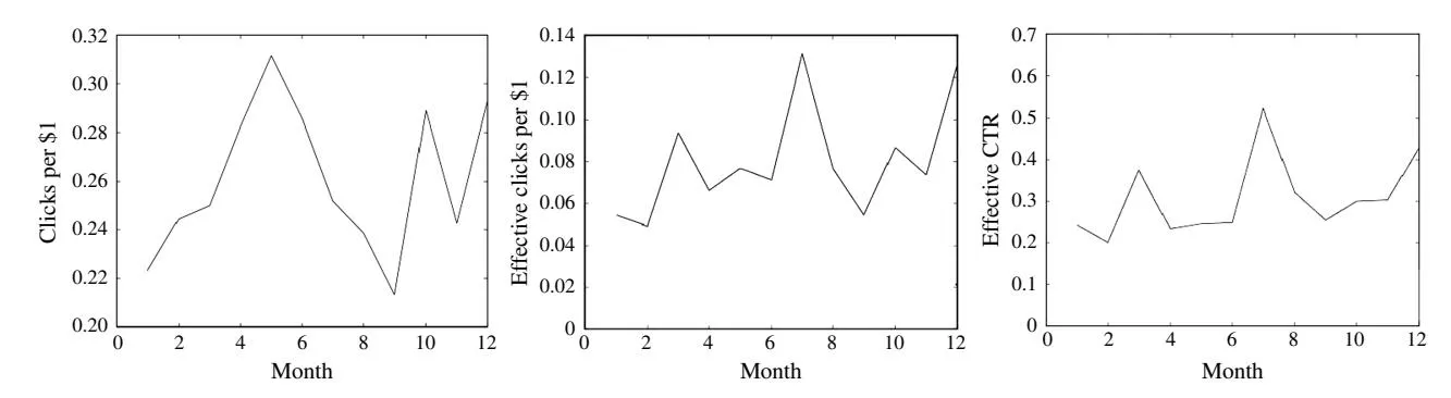
Figure 1 Clicks per Unit Budget, Effective Clicks per Unit Budget, and Effective CTR (at the Monthly Granularity)

respectively. The response constant is fixed at 0.04 in the following experiments.

5.2. Comparisons

We compared our budget allocation method (BOF-OC) with four baseline strategies. The first one represents the budget strategy from a type of advertisers who evenly allocate the budget across the two search markets and then over time (called BASE1-Average). The second baseline strategy first allocates the total budget across the two search markets according to the ratio of the gross advertising returns in each market; then the budget within a market is distributed over time based on our method (called BASE2-C-Ratio). The other two baseline strategies are derived from existing literature on bidding strategies, by treating the bidding decision for a single keyword as a special case of the budget decision. Because of the limited research on advertising budget allocation across several markets in sponsored search auctions, no existing research can be compared directly with ours. This is the reason we implemented the two baseline strategies derived from the literature on bidding strategies for comparison purposes.

Next, we describe how we derive these two baseline strategies. Let pⁱ 4t5 denote the advertiser’s bid price in market i at time t; then the objective function in model 3 can be given as

$\max \sum_{i} \int_{0}^{T} e^{-rt} \left( m_i(t) c_i(t) \theta_i(t) (v_i(t) - p_i(t)) \right) dt.$

In this model setting, bⁱ 4t1È5 = mⁱ 4t5cⁱ 4t5ⁱ 4t5pⁱ 4t5. That is, the bid price (i.e., pⁱ 4t5) can affect the market share (e.g., ) through bⁱ 4t1È5. The third baseline strategy (called BASE3-TB-Budget) is derived from the two-bid bidding strategy proposed in Feldman et al. (2007). The TB-Budget strategy distributes the budget in a market by randomly choosing between two values ^bi and ¯bⁱ over time; ^bi and ¯bⁱ correspond to the two bid prices determined by their two-bid strategy in market i, respectively. The fourth baseline strategy (called BASE4-CB-Budget) is derived from the cyclical bidding strategy proposed in Zhang and Feng (2011). The CB-Budget budget strategy distributes the budget based on a pulse function f over time, f 4t5 ∈ 6bⁱ 1 ¯bi 7.

$f(t + \Delta t) = \begin{cases} f(t) + \epsilon, & \text{if } f(t) < \bar{b}_i m; \\ \underline{b}_i, & \text{otherwise,} \end{cases}$

where denotes the increasing scale of the budget.

We execute two sets of experiments. One has lower gross advertising return (C¹ = 50, C² = 150, Figure 2), and the other has higher gross advertising return (C¹ = 100, C² = 300, Figure 3). We keep the advertising effort elasticity as a constant 0.05 in the two markets and the advertiser’s quality score q as 0.1.

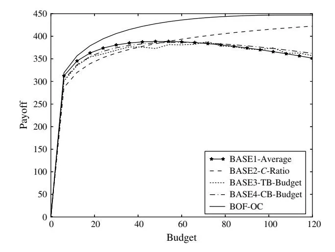
Figure 2 The Payoff of Five Strategies 4C¹ = 501 C² = 1505

Figures 2 and 3 show the payoff obtained by these five strategies at different (total) budget levels (B). From Figures 2 and 3, we observe the following:

• 1. In both cases, our strategy (BOF-OC) always outperforms the four baseline strategies.
• 2. In both cases, the payoff of the BASE1-Average, BASE3-TB-Budget, and BASE4-CB-Budget strategies initially increases and then exhibits a decreasing trend after a point. This is because the marginal revenue for an additional dollar invested (marginal cost) is decreasing as the budget increases. At a certain point, the marginal revenue will be smaller than the marginal cost; thus the marginal net payoff (i.e., the marginal revenue–marginal cost) will be negative, and the overall net payoff will decrease.
• 3. In both cases, the payoff generated by both BASE2-C-Ratio and our BOF-OC strategy first increases with the budget, then levels off. This is due to the existence of the producer equilibrium for these

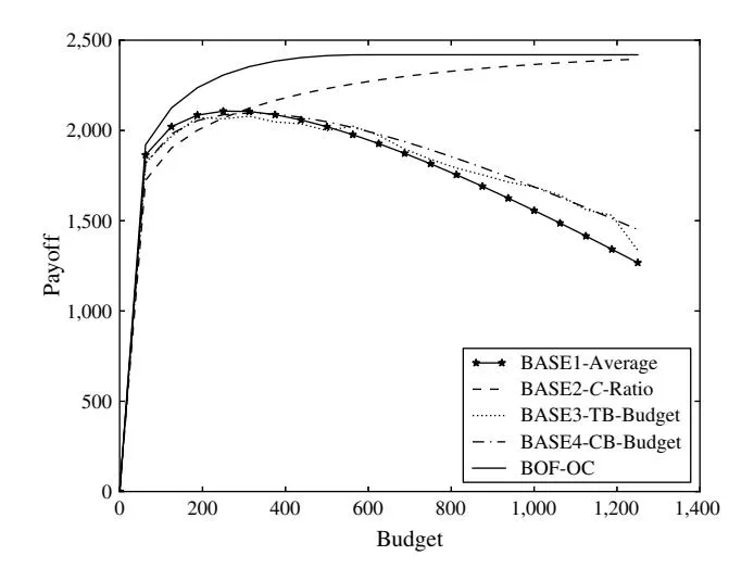
Figure 3 The Payoff of Five Strategies 4C¹ = 1001 C² = 3005

two strategies, where the marginal revenue equals the marginal cost.

4. The BASE3-TB-Budget and BASE4-CB-Budget strategies are superior to the BASE1-Average strategy and inferior to the BASE2-C-Ratio strategy as the total budget increases.

As we pointed out earlier, the setting of bidding strategies is quite different from that of budget decisions. These two have different decision variables. Our paper is the first to study budget decisions in such a dynamic setting, so there does not exist prior work that can be compared directly. The comparisons of the scaled-down problem show that our model performs better. However, we need to point out that this conclusion does not mean that our model is superior since a rigorous comparison needs to be based on exactly the same problem setting, which is not the case here.

5.3. Property Verification

We designed computational experiments to verify properties of our budget allocation method and conduct sensitivity analysis with respect to several important parameters. The data sets used in this section were generated from historical advertising logs. The experiments investigate how the advertising effort elasticity, the quality score, and the gross advertising return affect the optimal strategy and the corresponding payoff.

5.3.1. Influence of the Advertising Effort Elasticity . In the following experiments, we investigate the influence of different functional forms of on overall payoffs and study the budget allocations to different markets when the two markets have different . Specifically, we are intended to explore whether increasing the advertising effort elasticity over time will lead to more profit for an advertiser. According to Hax and Majluf (1982), as an advertiser accumulates more experience in the process of campaign management and promotion activities, her ability to make decisions (which is reflected through the advertising effort elasticity) improves. Then the same amount of advertising budget can result in a higher payoff.

Different forms of 0 We first consider three functional forms of advertising effort elasticity (). They have the same mean values. For each case, both markets have the same .

• Case 1a: constant between 601 T 7 (CONST, = 0005),
• Case 1b: linearly increasing between 601 T 7 (LINC, = 008t/T + 001),
• Case 1c: linearly decreasing between 601 T 7 (LDEC, = −008t/T + 009).

These three cases can represent three different types of advertisers. The CONST case represents mature advertisers with sufficient accumulated experience.

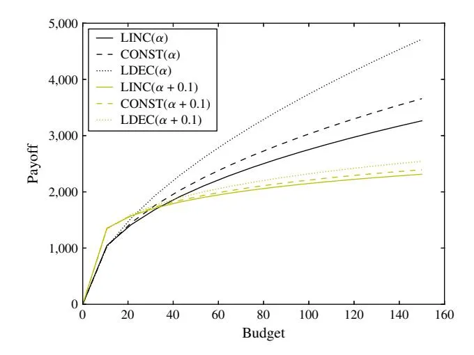
Figure 4 (Color online) The Payoff at Different Budget Levels in Three Shapes of Advertising Effort Elasticity

They have learned over time, and their ability to optimize advertising expenditure is stable. The LINC case represents advertisers who are relatively new to the market. They are still on a learning curve, and the advertising effort elasticity increases as they learn over time. The LDEC case represents advertisers whose effectiveness of converting advertising dollars to payoffs is declining for some internal or external reason (e.g., management change).

Figure 4 shows the payoff at different budget caps with these three forms of advertising effort elasticity and also the corresponding results when is increased by 0.1.

• (1) As shown in Figure 4, the payoffs of these three settings have the following relationship: LINC < CONST < LDEC. One possible explanation for this phenomenon is that higher advertising effort elasticity at an early stage will bring in more profit. This is true especially for the case with budget constraints. As the budget is draining off at late stages, advertisers are not able to allocate sufficient funds even if the elasticity increases. Thus, the advertiser with increasing elasticity is recommended to invest a higher share at later stages, but the advertiser with decreasing elasticity should invest a higher share at the initial stages to maximize net profits.
• (2) Comparing the three cases with +001 and the three cases without, we can clearly see that higher leads to higher payoffs.

Markets with Different 0 Here we allow different markets to have different values to study how the budget is allocated across the two markets based on the advertising effort elasticity.

• Case 2a: The advertiser’s effort elasticity is different in these two markets:

$\alpha_1(t) = 0.05 + 0.3\sin\frac{10\pi t}{T}$

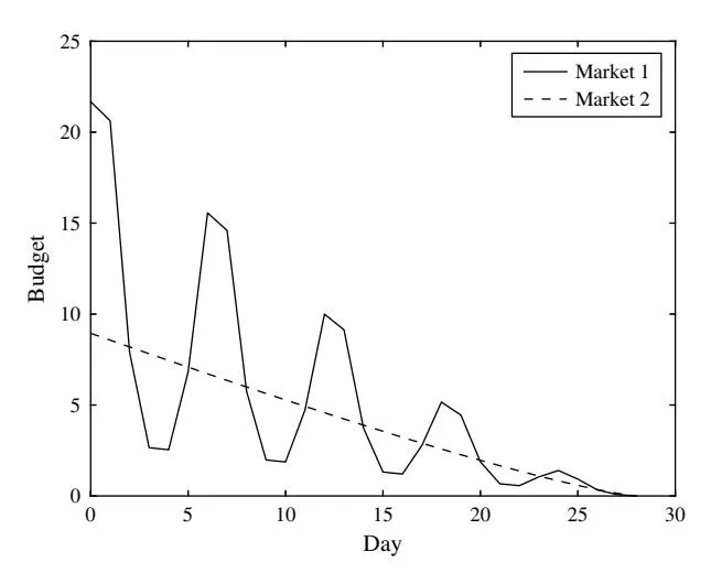
Figure 5 Optimal Budget Allocated to Two Search Markets Over Time in Case 2a

in search market 1 (i.e., the advertiser’s elasticity experiences ups and downs over time), and ² 4t5 = 0005 in market 2 (i.e., the advertiser’s elasticity stays constant over time).

• Case 2b: The advertiser’s effort elasticity stays the same over time and across two markets, i.e., 1 4t5 = ² 4t5 = 0005.

Figures 5 and 6 illustrate the optimal budget allocated to the two search markets over time under these two cases, respectively. When the two markets have the same (Figure 6), the optimal budgets allocated to the two markets are almost the same. When the two markets have different (Figure 5), the optimal budgets allocated to the two markets are significantly different. As the advertiser’s elasticity experiences ups and downs over time, so does the budget allocation. Thus, we can draw the conclusion that the advertising effort elasticity has a significant influence on the optimal budget allocation in the two markets.

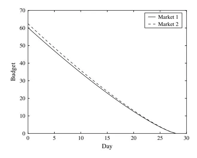
Figure 6 Optimal Budget Allocated in Two Search Markets Over Time in Case 2b

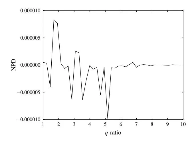
Figure 7 The Normalized Performance Difference in Case 3a

5.3.2. Influence of q. In this experiment, we first study the influence of the quality score (q) on the optimal payoff. Since each market has a quality score, we study how the ratio q1/q² affects the optimal payoff. We study the influence of q1/q² under two settings, one with low gross advertising return (Case 3a: C¹ = C² = 50) and the other with high gross advertising return (Case 3b: C¹ = C² = 200). Under each setting, we first compute the payoff generated by the C ratiobased strategy (i.e., BASE2-C-Ratio), and then calculate the normalized payoff difference (NPD) between the payoff from BASE2-C-Ratio and the payoff of our BOF-OC strategy. NPD is defined as 4f² − f¹ 5/f¹ , where f¹ and f² represent the payoff by BASE2-C-Ratio and by our approach, respectively. The reason we use NPD instead of the payoff generated by our BOF-OC is that NPD provides a relative change of the payoff from BOF-OC. The payoff from the BASE2-C-Ratio method does not change when C (C¹ and C² ) is fixed. As NPD becomes smaller or bigger, so does the payoff from our BOF-OC strategy.

Figures 7 and 8 show the normalized payoff difference for Cases 3a and 3b as q1/q² increases from 1 to 10.

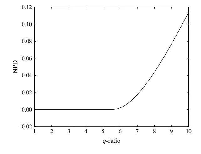
Figure 8 The Normalized Performance Difference in Case 3b

As shown in Figure 7, the quality score ratio between these two markets (q-ratio) has a negligible (e.g., the scale of NPD is 0.000005) and unstable effect on the optimal budget strategy (case 3a). This implies that the effect of q on the market share and the optimal budget strategy is unclear when C is relatively small. Note that the small NPD in Case 3a indicates that the payoff from our BOF-OC method does not change much with q-ratio.

As shown in Figure 8, in Case 3b there exists an interval (1 ≤ q1/q² ≤ 6) where q-ratio has a negligible effect (NPD ≈ 0). However, q begins to increasingly influence the optimal budget strategy when q1/q² ≥ 6. This implies that q has some effect on the optimal budget strategy only when its ratio across markets is large enough to influence the market share in the situation where C is large.

5.3.3. The Influence of Gross Advertising Return C. In this experiment, we investigate the influence of different C values and the ratio of C¹ and C² in two markets.

Different C Value0 As shown in Figures 7 and 8, different C values do have some effect on the payoff. In this experiment, we want to study how the change in C affects the NPD. We increase C¹ and C² together while keeping C1/C² = 3. Figure 9 shows the NPD with C¹ increasing from 0 to 3,000.

As shown in Figure 9, the payoff from the BASE2- C-Ratio method is very close to that from our BOF-OC solution when C (C¹ and C² ) is small (NPD ≈ 0 region). This indicates that we can use the BASE2- C-Ratio method to approximate the optimal solution when C (C¹ and C² ) is relatively small. We investigate this further in the next section.

Ratio of C¹ and C² 0 As shown in Figure 9, C does not seem to have a significant effect on the payoff when it is relatively small. That is, using C-ratio alone is

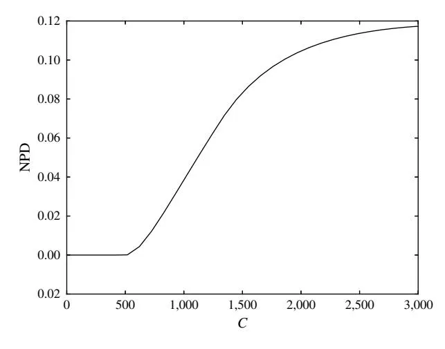
Figure 9 The Normalized Performance Difference with C1/C² = 3

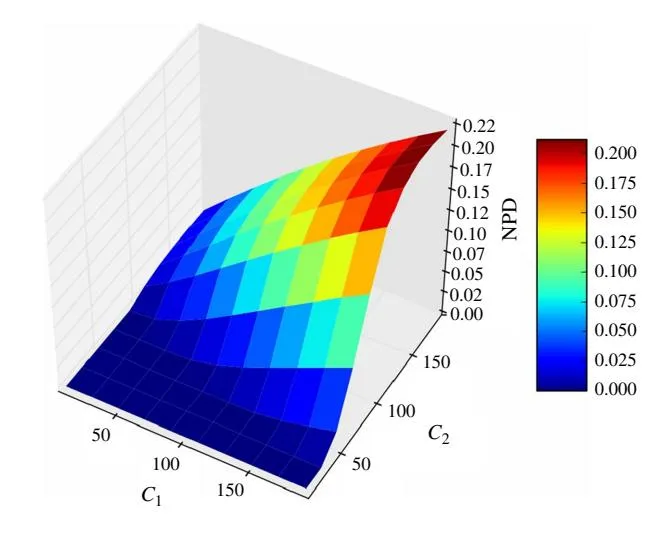
Figure 10 (Color online) The Normalized Performance Difference with Varying C¹ and C²

enough to derive a near-optimal solution (the BASE2- C-Ratio method). In this section, we further investigate the relationship between C and the NPD varying both C¹ and C² .

From Figure 10, we can draw the following conclusions.

• (1) On the surface of normalized payoff difference, there exist two quite distinct regions. The first region is called the C-sensitive region, where either C¹ or C2 is small; the second region is called the C-insensitive region, where both C¹ and C² are large. In the C-sensitive region, we can use BASE2-C-Ratio method to approximate the optimal solution, but we cannot do that in the C-insensitive region.
• (2) It also proves an interesting property of our budget model—when the gross advertising return is relatively small, the ratio of optimal budgets allocated to these two search markets approximates the ratio of gross advertising returns in these two markets, e.g., B1 2 B² ≈ C¹ 2 C² . Thus, an advertiser can simply use the C ratio-based strategy, which could have nearoptimal performance in cases with smaller C and a constrained advertising budget.
• (3) In summary, in the C-sensitive region, C has a dominating influence on the optimal budget strategy, whereas other factors (such as q and ) have insignificant effects. The reason might be that the change in these other factors is inadequate to influence market share in the C-sensitive situation.

5.4. Managerial Insights

Our research provides several managerial insights for advertisers in sponsored search advertising.

First, as demonstrated through both theoretical analysis and experimental evaluation, the optimal

budget allocation solution would be quite different for the two cases—with or without budget constraints. Moreover, different levels of the total marketlevel advertising budget can lead to different optimal strategies and payoffs. This indicates that an advertiser should allocate her budget in a different manner depending on the amount of budget available to her in a certain promotional period. Often times, in practice, the same allocation strategy is adopted.

Second, there exists a producer equilibrium where the marginal payoff (i.e., the net profit generated by one additional unit of advertising expenditure) is zero (Theorem 2). In other words, in the equilibrium there won’t be any additional payoff from increasing advertising expenditure. This phenomenon implies that there exists a saturation level of advertising expenditure in the sponsored search market. Specifically, below this saturation level, adding funds will lead to additional payoff, whereas at (or over) this level, increasing funds will not result in additional payoff. This also coincides with the law of diminishing marginal utility in economics. Therefore, advertisers should estimate when the saturation level will be reached and cautiously make budget decisions to avoid overspending.

Third, in the C-sensitive region (i.e., the gross advertising return in either search market is relatively small), the gross advertising return has a dominating effect on the optimal strategy and corresponding payoffs. In other words, using only C to allocate the budget (the C ratio-based strategy) will lead to a near-optimal result in the C-sensitive region. This indicates that when the gross advertising return of search markets is relatively small, advertisers can use a simple C ratio-based method to help them allocate their budget. When C is large in both markets, advertisers should incorporate all the factors such as the total budget, quality score, and advertising effort elasticity to make the optimal decision. According to the definition of the composite factor C, the C-sensitive situation occurs when (1) the advertiser is from a small company or (2) the size of the target population in a search market is small. Therefore, this provides a simple but effective heuristic strategy for budget allocation for small business advertisers. However, the precise determination of the value range and boundaries of these factors demands a comprehensive empirical study that is beyond the scope of this paper.

Finally, experiments with different forms of advertising effort elasticity suggest that advertisers with increasing advertising effort elasticity are recommended to invest higher shares at the later stages, whereas those with decreasing advertising effort elasticity should invest higher shares at the initial stages to maximize net profit.

6. Practical Implementation Issues

In this section we discuss several issues related to the possible implementation of our solution in real sponsored search advertising campaigns.

Our paper provides a solution process to derive the optimal budget strategy for search advertising across markets over a given promotional period. For an advertiser with a total budget B, Algorithm 1 is first used to derive the optimal budget solution (without considering B as the budget constraint). If the sum of the optimal budgets over the entire promotional period is smaller than the total budget B (the case without budget constraints), the advertiser can adopt the solution from Algorithm 1 as the final optimal budget strategy (Equation (7)). If the sum of the optimal budgets over the entire promotional period is bigger than the total budget B (the case with budget constraints), Algorithm 2 is then used to derive the final optimal budget solution (Equation (8)).

For both cases, the advertiser needs to estimate the following five parameters necessary for making budget allocation decisions: the potential search demand m, the proportion of effective clicks c, the value-per-click v, the quality score q, and the advertising effort elasticity . Next we provide some insights for estimating these parameters in real-world search advertising budget decision settings.

• The potential search demand in a search market can be obtained from keyword research tools provided by major search engines or third-party companies (e.g., WordTracker). For example, Google AdWords provides the information about the number of online searches conducted by search users over the past month for a specific keyword or phrase. Through continuous observations over time for a certain set of keywords, a search demand curve can be generated. In a similar way, Google Trends also provides a search demand curve for a given keyword. In this work, to provide more accurate evaluation, we obtain the search demand for a set of keywords based on historical data from Google Trends. However, for advertisers who are allocating budgets for future search advertising campaigns, we recommend they employ a prediction model to estimate the future search demand based on the time series data. The double seasonal multiplicative ARIMA model (Mohamed et al. 2010) is a good predictive model to consider because of the presence of a double seasonal pattern in the time series data (i.e., daily and weekly seasonality).
• The value-per-click and the proportion of effective clicks in a search market can be estimated from historical reports and logs of advertising campaigns and the advertiser’s proprietary information. The value-per-click is related to the advertiser’s proprietary information, such as the cost and price of the product or service, and can be easily determined. For

an advertiser who has conducted advertising campaigns previously, an appropriate set of predictor variables (e.g., impression, rank, click-through rate, and search users’ activities on the advertiser’s website) are recorded in the historical logs and reports. Then a Bayesian probit regression model can be used to dynamically learn and predict the effective proportion of clicks of future search advertising campaigns (Graepel et al. 2010).

• Because of the proprietary nature of search engine operations, it is impossible to obtain the quality score (q) directly from the advertiser. In this work we take the CTR as the quality score in the comparison experiment. In practice, we can also measure the relevance between the ad text and the corresponding landing page, between the keyword and the ad text, between the keyword and the query using text mining techniques (e.g., Raghavan and Hillard 2009). An advertiser’s quality score can then be approximated as the product of her CTR and the relevance factors. In the situation with stable advertising performance, the quality score’s amplitude of variation is quite small. Therefore, it can be treated as a constant during a given promotional period.
• The advertising effort elasticity can be instantiated as the normalized profit-per-unit cost. Usually, it is reasonable to assume that the advertising effort elasticity is either stable during a short period of time or increasing slowly during a long period of time because the advertiser’s ability to leverage advertising dollars usually increases with the experience accumulation of advertising operations.

These parameters can be first initialized based on historical reports in the ways described previously. After each advertising period, the advertiser should observe the state variable (i.e., the market share ) that can be easily obtained from the number of impressions and search demand in a specific period and also must update the five parameters continuously by tracking the ongoing advertising performance. As the estimations get more and more accurate, the budget allocation decisions can also be improved over time.

There is one additional insight observed from the experiments. As we discuss in §5.4, when the gross advertising return in either search market is relatively small, advertisers can use the C ratio-based strategy to reach near-optimal budget allocations. Specifically, the advertiser can first allocate the total budget across the search markets according to the ratio of the gross advertising returns from each market, and then the budget allocated to each market is distributed over time based on our method. This applies mostly to advertisers with a small target population in a search market. This can be meaningful in practice since such a simple heuristic strategy gives small advertisers with limited resources a chance to consider optimizing their budget decisions.

7. Conclusions and Future Directions

In this paper we present a novel optimal budget allocation model to dynamically allocate the advertising budget across several search markets simultaneously, under a finite time horizon. Our model captures several distinctive features of sponsored search advertising by introducing dynamic advertising effort u and quality score q to extend the advertising response function to suit search advertising scenarios. We also discuss a range of properties and present a feasible solution for our model. We have conducted a series of computational experiments to evaluate our model and identified properties, performed sensitivity analysis with respect to several important parameters, and validated our strategy by comparing it with four baseline strategies based on real-world data from actual advertising campaigns. Experimental results show that our strategy outperforms these four baseline strategies. Our research brings out some critical managerial insights for advertisers in conducting sponsored search advertising: (1) there exists a producer equilibrium where the marginal payoff is zero, and different levels of advertising budget will lead to different optimal strategies and payoffs; (2) advertisers with increasing advertising effort elasticity should invest higher shares in later stages of the marketing campaign, whereas those with decreasing advertising effort elasticity should invest higher shares in the earlier stages; and (3) the gross advertising return has a dominating effect on the optimal strategy in the C-sensitive region.

We are in the process of extending our model in the following directions: (a) a comprehensive empirical study of our budget approach to validate identified properties and to determine the value range and boundaries of impact factors in field experiments of search campaigns, (b) budget allocation strategies in uncertain marketing environments of sponsored search auctions, and (c) further refinements of the proposed algorithm to improve space and time efficiencies, with the aim of developing practical online budget allocation decision-making tools.

Supplemental Material

Supplemental material to this paper is available at http://dx .doi.org/10.1287/ijoc.2014.0626.

References

• Abrams Z, Mendelevitch O, Tomlin J (2007) Optimal delivery of sponsored search advertisements subject to budget constraints. Proc. 8th ACM Conf. Electronic Commerce (ACM, New York), 272–278.

• Amin K, Kearns M, Key P, Schwaighofer A (2012) Budget optimization for sponsored search: Censored learning in MDPs. 28th Conf. Uncertainty Artificial Intelligence (AUAI Press, Catalina Island, CA), 54–63.

• Aravindakshan A, Naik P (2011) How does awareness evolve when advertising stops? The role of memory. Marketing Lett. 22(3):315–326.

• Berkowitz D, Allaway A, D’Souza G (2001) Estimating differential lag effects for multiple media across multiple stores. J. Advertising 30(4):59–65.

• Bertsekas DP (1995) Dynamic Programming and Optimal Control, Vol. 1 (Athena Scientific, Belmont, MA).

• Du R, Hu Q, Ai S (2007) Stochastic optimal budget decision for advertising considering uncertain sales responses. Eur. J. Oper. Res. 183(3):1042–1054.

• Erickson GM (1992) Empirical analysis of closed-loop duopoly advertising strategies. Management Sci. 38(12):1732–1749.

• Feldman J, Muthukrishnan S, Pal M, Stein C (2007) Budget optimization in search-based advertising auctions. Proc. 9th ACM Conf. Electronic Commerce (ACM, New York), 40–49.

• Feng J, Bhargava HK, Pennock DM (2007) Implementing sponsored search in Web search engines: Computational evaluation of alternative mechanisms. INFORMS J. Comput. 19(1):137–148.

• Fischer M, Albers S, Wagner N, Frie M (2011) Dynamic marketing budget allocation across countries, products, and marketing activities. Marketing Sci. 30(4):568–585.

• Fruchter GE, Dou W (2005) Optimal budget allocation over time for keyword ads in Web portals. J. Optim. Theory Appl. 124(1): 157–174.

• Fuller AT (1963) Bibliography of Pontryagin’s maximum principle. J. Electronics Control 15(5):513–517.

• Google Inc. (2014) 2014 financial tables. Accessed September 16, 2014, http://investor.google.com/financial/tables.html.

• Graepel T, Candela JQ, Borchert T, Herbrich R (2010) Web-scale Bayesian click-through rate prediction for sponsored search advertising in Microsoft’s Bing search engine. Proc. 27th Internat. Conf. Machine Learn. (ICML-10), 13–20.

• Gummadi R, Key PB, Proutiere A (2011) Optimal bidding strategies in dynamic auctions with budget constraints. Comm., Control, Comput. (Allerton), 2011 49th Annual Allerton Conf., Haifa, Israel, 588.

• Hax AC, Majluf NS (1982) Competitive cost dynamics: The experience curve. Interfaces 12(5):50–61.

• Holthausen JDM, Assmus G (1982) Advertising budget allocation under uncertainty. Management Sci. 28(5):487–499.

• Krishnamoorthy A, Prasad A, Sethi SP (2010) Optimal pricing and advertising in a durable-good duopoly. Eur. J. Oper. Res. 200(2):486–497.

• Little JDC (1979) Aggregate advertising models: The state of the art. Oper. Res. 27(4):629–667.

• Mohamed N, Ahmad MH, Ismail Z, Suhartono S (2010) Double seasonal ARIMA model for forecasting load demand. Matematika 26(2):217–231.

• Muthukrishnan S, Pál M, Svitkina Z (2010) Stochastic models for budget optimization in search-based advertising. Algorithmica 58(4):1022–1044.

• Naik PA, Mantrala MK, Sawyer AG (1998) Planning media schedules in the presence of dynamic advertising quality. Marketing Sci. 17(3):214–235.

• Nerlove M, Arrow KJ (1962) Optimal advertising policy under dynamic conditions. Economica 29(114):129–142.

• Özlük Ö, Cholette S (2007) Allocating expenditures across keywords in search advertising. J. Revenue Pricing Management 6(4): 347–356.

• Raghavan H, Hillard D (2009) A relevance model based filter for improving ad quality. Proc. 32nd Internat. ACM SIGIR Conf. Res. Development Inform. Retrieval (ACM, New York), 762–763.

• Rao AG, Rao MR (1983) Optimal budget allocation when response is S-shaped. Oper. Res. Lett. 2(5):225–230.

• Sasieni MW (1971) Optimal advertising expenditure. Management Sci. 18(4, Part II):P-64–P-72.

• Search Engine Watch (2006) The search engine report—Number 117. Accessed September 16, 2014, http://searchenginewatch.com/ article/2064122/The-Search-Engine-Report-Number-117.

• Sethi SP (1973) Optimal control of the Vidale-Wolfe advertising model. Oper. Res. 21(4):998–1013.

• Sethi SP (1977) Dynamic optimal control models in advertising: A survey. SIAM Rev. 19(4):685–725.

• Sethi SP (1983) Deterministic and stochastic optimization of a dynamic advertising model. Optimal Control Appl. Methods 4(2):179–184.

• Sethi SP, Thompson GL (2000) Optimal Control Theory: Applications to Management Science and Economics, 2nd ed. (Springer, New York).

• Sethi SP, Prasad A, He X (2008) Optimal advertising and pricing in a new-product adoption model. J. Optim. Theory Appl. 139(2): 351–360.

• Sorger G (1989) Competitive dynamic advertising: A modification of the case game. J. Econom. Dynam. Control 13(1):55–80.

• Sutherland M (2009) Advertising and the Mind of the Consumer (Allen & Uwin, St. Leonards, NSW, Australia).

• Tull DS, Wood VR, Duhan D, Gillpatrick T, Robertson KR, Helgeson JG (1986) “Leveraged” decision making in advertising: The flat maximum principle and its implications. J. Marketing Res. 23(1):25–32.

• Varian H (2006) The economics of Internet search. Rivista di Politica Economica 96(11/12):177–191.

• Vidale ML, Wolfe HB (1957) An operations-research study of sales response to advertising. Oper. Res. 5(3):370–381.

• Yang Y, Zhang J, Qin R, Li J, Liu B, Liu Z (2013) Budget optimization strategies in uncertain environments of search auctions: A preliminary investigation. IEEE Trans. Services Comput. 6(2): 168–176.

• Yang Y, Zhang J, Qin R, Li J, Wang F, Qi W (2012) A budget optimization framework for search advertisements across markets. IEEE Trans. Systems, Man, Cybernetics, Part A 42(5):1141–1151.

• Yao S, Mela CF (2011) A dynamic model of sponsored search advertising. Marketing Sci. 30(3):447–468.

• Zhang X, Feng J (2005) Price cycles in online advertising auctions. Proc. 26th Internat. Conf. Inform. Systems (ICIS), Las Vegas, NV, 769–781.

• Zhang X, Feng J (2011) Cyclical bid adjustments in search-engine advertising. Management Sci. 57(9):1703–1719.