Predicting Advertiser Bidding Behaviors In Sponsored Search

ABSTRACT

We study how an advertiser changes his/her bid prices in sponsored search, by modeling his/her rationality. Predicting the bid changes of advertisers with respect to their campaign performances is a key capability of search engines, since it can be used to improve the offline evaluation of new advertising technologies and the forecast of future revenue of the search engine. Previous work on advertiser behavior modeling heavily relies on the assumption of perfect advertiser rationality; however, in most cases, this assumption does not hold in practice. Advertisers may be unwilling, incapable, and/or constrained to achieve their best response. In this paper, we explicitly model these limitations in the rationality of advertisers, and build a probabilistic advertiser behavior model from the perspective of a search engine. We then use the expected payoff to define the objective function for an advertiser to optimize given his/her limited rationality. By solving the optimization problem with Monte Carlo, we get a prediction of mixed bid strategy for each advertiser in the next period of time. We examine the effectiveness of our model both directly using real historical bids and indirectly using revenue prediction and click number prediction. Our experimental results based on the sponsored search logs from a commercial search engine show that the proposed model can provide a more accurate prediction of advertiser bid behaviors than several baseline methods.

Keywords

Advertiser modeling, rationality, sponsored search, bid prediction. [Information Systems]: Information Storage and Retrieval - On-line Information Services

1. INTRODUCTION

Sponsored search has become a major means of Internet monetization, and has been the driving power of many commercial search engines. In a sponsored search system, an advertiser creates a number of ads and bids on a set of keywords (with certain bid prices) for each ad. When a user submits a query to the search engine, and if the bid keyword can be matched to the query, the corresponding ad will be selected into an auction process. Currently, the Generalized Second Price (GSP) auction [10] is the most commonly used auction mechanism which ranks the ads according to the product of bid price and ad click probability¹ and charges an advertisers if his/her ad wins the auction (i.e., his/her ad is shown in the search result page) and is clicked by users [13].

Generally, an advertiser has his/her goal when creating the ad campaign. For instance, the goal might be to receive 500 clicks on the ad during one week. However, the way of achieving this goal might not be smooth. For example, it is possible that after one day, the ad has only received 10 clicks. In this case, in order to improve the campaign performance, the advertiser may have to increase the bid price in order to increase the opportunity for his/her ad to win future auctions, and thus to increase the chance for the ad to be presented to users and to be clicked.²

Predicting how the advertisers change their bid prices is a key capability of a search engine, since it can be used to deal with the so-called second order effect in online advertising [13] when evaluating novel advertising technologies and forecasting future revenue of search engines. For instance, suppose the search engine wants to test a novel algorithm for bid keyword suggestion³ [7]. Given that the online experiments are costly (e.g., unsuccessful online experiments will lead to revenue loss of the search engine), the algorithm will usually be tested based on the historical logs first to see its ef-

^∗This work was performed when the first and the third authors were interns at Microsoft Research Asia.

¹Usually a reserve score is set and the ads whose scores are greater than the reserve score are shown.

²Note that the advertiser may also choose to revise the ad description, bid extra keywords, and so on. However, among these actions, changing the bid price is the simplest and the most commonly used method by advertisers. Please also note that since GSP is not incentive compatible, advertisers might not bid their true values and changing bid prices is their common behaviors.

³The same thing will happen when we evaluate other algorithms like traffic estimation, ad click prediction, and auction mechanism.

fectiveness (a.k.a., offline experiment). However, in many cases, even if the algorithm works quite well in offline experiment, it may perform badly after being deployed online. One of the reasons is that the advertisers might change their bid prices in response to the changes of their campaign performances caused by the deployed new algorithm. Therefore, the experiments based on the historical bid prices will be different from those on online traffic. To tackle this problem, one needs a powerful advertiser behavior model to predict the bid price changes.

In the literature, there have been a number of researches [4] [5] [22] [19] [2] [17] [3] that model how advertisers determine their bid prices, and how their bid strategies influence the equilibrium of the sponsored search system. For example, Varian [19] assumes that the advertisers bid the amount at which their value per click equals the incremental cost per click to maximize their utilities. The authors of [2] and [17] study how to estimate value per click, by assuming advertisers are on the locally envy-free equilibrium, and assuming the distributions of all the advertisers’ bids are independent and identically distributed.

Most of the above researches rely highly on the assumptions of perfect advertiser rationality and full information access⁴ , i.e., advertisers have good knowledge about their utilities and are capable of effectively optimizing the utilities (i.e., take the best response). However, as we argue in this paper, this is usually not true in practice. In our opinion, real-world advertisers have limitations in accessing the information about their competitors, and have different levels of rationality. In particular, an advertiser may be unwilling, incapable, or constrained to achieve his/her “best response.” As a result, some advertisers frequently adjust the bid prices according to their recent campaign performances, while some other advertisers always keep the bid unchanged regardless of the campaign performances; some advertisers have good sense of choosing the appropriate bid prices (possibly with the help of campaign analysis tools [14] or third-party ad agencies), while some other advertisers choose bid prices at random.

To better describe the above intuition, we explicitly model the rationality of advertisers from the following three aspects:

Willingness represents the propensity an advertiser has to optimize his/her utility. Advertisers who care little about their ad campaigns and advertisers who are very serious about the campaign performance will have different levels of willingness.
Capability describes the ability of an advertiser to estimate the bid strategies of his/her competitors and take the bestresponse action on that basis. An experienced advertiser is usually more capable than an inexperienced advertiser; an advertiser who hires professional ad agency is usually more capable than an advertiser who adjusts bid prices by hisself/herself.
Constraint refers to the constraints that prevent an advertiser from adopting a bid price even if he/she knows that this bid price is the best response for him/her. The constraint usually (although not only) comes from the lack of remaining budget.

With the above notions, we propose the following model to describe how advertisers change their bid prices, from the perspective of the search engine.⁵ First, an advertiser has a certain probability to optimize his/her utility or not, which is modeled by the willingness function. Second, if the advertiser is willing to make changes, he/she will estimate the bid strategies of his/her competitors. Based on the estimation, he/she can compute the expected payoff (or utility) and use it as an objective function to determine his/her next bid price. This process is modeled by the capability function. By simultaneously considering the optimization processes of all the advertisers, we can effectively compute the best bid prices for every advertiser. Third, given the optimal bid price, an advertiser will check whether he/she is able to adopt it according to some constraints. This is modeled by the constraint function.

Please note that the willingness, capability, and constraint functions are all parametric. By fitting the output of our proposed model to the real bid change logs (obtained from commercial search engines), we will be able to learn these parameters, and then use the learned model to predict the bid behavior change in the future. We have tested the effectiveness of the proposed model using real data. The experimental results show that the proposed model can predict the bid changes of advertisers in a more accurate manner than several baseline methods.

To sum up, the contributions of our work are listed as below. First, to the best of our knowledge, this is the first advertiser behavior model in the literature that considers different levels of rationality of advertisers. Second, we model advertiser behaviors using a parametric model, and apply machine learning techniques to learn the parameters in the model. This is a good example of leveraging machine learning in game theory to avoid its unreasonable assumptions. Third, our proposed model leads to very accurate bid prediction. In contrast, as far as we know, most of previous research focuses on estimating value per click, but not predicting bid prices. Therefore, our work has more direct value to search engine, given that bid prediction is a desired ability of search engine as aforementioned.

The rest of the paper is organized as the following. In Section 2, we introduce the notations and describe the willingness, capability, and constraint functions. We present the framework of the bid strategy prediction model in Section 3. In Section 4, we introduce the efficient numerical algorithm of the model. In Section 5, we present the experimental results on real data. We summarize the related work in Section 6, and in the end we conclude the paper and present some insights about future work in Section 7.

2. ADVERTISER RATIONALITY

As mentioned in the introduction, how an advertiser adjusts his/her bid is related to his/her rationality. In our opinion, there are three aspects to be considered when modeling the rationality of an advertiser: willingness, capability, and constraint. In this section, we introduce some notations for sponsored search auctions, and then describe the models for these rationality aspects.

2.1 Notations

We consider the keyword auction in sponsored search. For simplicity, we will not consider connections between different ad campaigns and we assume each advertiser only has one ad and bids on just one keyword for it. That is, the auction participants are the keyword-ad pairs. Advertisers are assumed to be risk-neutral.⁶

⁴ Please note that some of these works take a Bayesian approach; however, they still assume that the priors of the value distributions are publicly known.

⁵That is, the model is to be used by the search engine to predict advertisers’ behavior, but not by the advertisers to guide their bidding strategies.

⁶This assumption will result in a uniform definition of utility functions for all the advertisers. However, our result can be naturally

We use i ( $i = 1, \dots, I$ ) to index the advertisers, and consider advertiser l as the default advertiser of our interest. Suppose in one auction the advertisers compete for J ad slots. In practice, the search engine usually introduces a reserve score to optimize its revenue. Only those ads whose rank scores are above this reserve score will be shown to users. To ease our discussion, we regard the reserve score r as a virtual advertiser in the auction. We use $a_{i,j}$ to denote the click-through rate (CTR) of advertiser i’s ad when it is placed at position j. Similar to the setting in [2][17], we assume $a_{i,j}$ to be separable. That is, $a_{i,j} = \gamma_i \alpha_j$ , where $\gamma_i$ is the ad effect and $\alpha_j$ is the position effect. We let $\alpha_j = 0$ when j > J. The sponsored search system will predict the click probability [11] of an ad and use it as a factor to rank the ads in the auction. We use $s_i$ to denote the predicted click probability of advertiser i’s ad if it is placed in the first ad slot. Note that both $a_{i,j}$ and $s_i$ are random variables [2], since they may be influenced by many dynamic factors such as the attributes of the query and the user who issues the query.

We assume all the advertisers share the same bid strategy space $\Omega$ which consists of B different discrete bid prices denoted by $b_i, i=1,\cdots,B$ . Furthermore, we denote the strategy of advertiser l as $\pi_l=(\pi_{l,1},\cdots,\pi_{l,B})$ , which is a mixed strategy. It means that l will use bid strategy $b_i$ with a probability of $\pi_{l,i}, i=1,\cdots,B$ . We assume advertiser l will estimate both the configuration of his/her competitors and their strategies in order to find his/her own best response. We use $\mathbb S$ (including l) to indicate the set of advertisers who are regarded by advertiser l as the participates of the auction and use $\mathbb S_{-l}$ (excluding l) to indicate the set of competitors of l. We denote $\pi_i^{(l)}$ as l’s estimated bid strategy for a competitor i ( $i \neq l$ ), and denote l’s own best-response strategy as $\pi_l^{(l)}$ .

Note that both $\mathbb S$ and $\pi_i^{(l)}(i\neq l)$ are random: (i) $\mathbb S$ is a random set due to the uncertainty in the auction process: a) the participants of the auction is dynamic [17]; b) in practice l never knows exactly who are competing with him/her since such information is not publicly available. (ii) $\pi_i^{(l)}(i\neq l)$ is a random vector due to l’s incomplete information and our uncertainty on l’s estimation. More intuitions about $\pi_i^{(l)}$ will be explained in the modeling of the capability function (see Section 2.3).

To ease our discussion, we now transform the uncertainty of $\mathbb S$ to the uncertainty in bid prices, as shown below. That is, we regard all the other advertisers as the competitors of l and add the zero bid price (denoted by $b_0$ ) to extend the bid strategy space. The extended bid strategy space is represented by $\Omega^* = \Omega \bigcup \{b_0\}$ . If an advertiser is not a real competitor of l, we regard his/her bid price to be zero. According to the above discussion, $\mathbb S$ will be the whole advertiser set with the set size I. Thus, we will only consider the uncertainty of bid prices in the rest of the paper.

2.2 Willingness

Willingness represents the propensity an advertiser is willing to optimize his/her utility, which is modeled as a possibility. We model willingness as a logistic regression function $W_l(\boldsymbol{x}_t^{(l)})$ . Here the input $\boldsymbol{x}_t^{(l)} = (x_{t,1}^{(l)}, \cdots, x_{t,H}^{(l)})$ is a feature vector (H is the number of features) extracted for advertiser l at period t, and the output is a real number in [0,1] representing the probability that l will optimize his/her utility. That is, advertiser l with feature vector $\boldsymbol{x}_t^{(l)}$

extended to the case where advertisers’ different risk preferences are considered.

will have a probability of $W_l(\boldsymbol{x}_t^{(l)})$ to optimize his/her utility, and a probability of $1 - W_l(\boldsymbol{x}_t^{(l)})$ to take no action.

In order to extract the feature vector $\boldsymbol{x}_{t}^{(l)}$ , we split the historical auction logs into T periods (e.g., T days). For each period $t \in$ $T,\,y_t^{(l)}$ indicates whether the bid was changed in period t+1. If the bid was changed, $y_t^{(l)}=1$ ; otherwise, $y_t^{(l)}=0$ . With this data, the following features are extracted: (i) The number of bid changes before t. The intuition is that an advertiser who changes bid more frequently in the past will also have a higher possibility to make changes in the next period. (ii) The number of periods that an advertiser has kept the bid unchanged until t. Intuitively, an advertiser who has kept the bid unchanged for a long time may have a higher possibility to continue keeping the bid unchanged. (iii) The number of different bid values used before t. The intuition is that an advertiser who has tried more bid values in the past may be regarded as a more active bidder, and we may expect him/her to try more new bid values in the future. (iv) A Boolean value indicating whether there are clicks in t. The intuition is that if there is no click, the advertiser will feel unsatisfied and thus have a higher probability to make changes.

With the above features, we write the willingness function as,

$W_l(\boldsymbol{x}_t^{(l)}) = \frac{1}{1 + e^{\{\beta_0^{(l)} + \sum_{n=1}^H \beta_n^{(l)} x_{t,n}^{(l)}\}}}, \ (t = 1, \cdots, T).$

Here $m{\beta}^{(l)}=(eta_0^{(l)},\cdots,eta_H^{(l)})$ is the parameter vector for l.

To learn the parameter vector $\boldsymbol{\beta}^{(l)}$ , we minimize the sum of the first-order error $\sum_{t=1}^{T}|y_t^{(l)}-W_l(\boldsymbol{x}_t^{(l)})|$ on the historical data using the classical Broyden-Fletcher-Goldfarb-Shanno algorithm (BFGS) [15]. Then we apply the learned parameter $\boldsymbol{\beta}^{(l)}$ to predict l’s willingness of change in the future.

2.3 Capability

Capability describes the ability of an advertiser to estimate the bid strategies of his/her competitors and take the best-response action on that basis. A more experienced advertiser may have better capability in at least three aspects: information collection, utility function definition, and utility optimization. Usually, in GSP auctions, a standard utility function is used and the optimal solution is not hard to obtain. Hence, we mainly consider the capability in information collection, i.e., the ability in estimating competitors’ bid strategies

Recalling that l does not have any exact information on his/her competitors’ bids, it is a little difficult to model how advertiser l estimates his/her competitors’ strategies, because different l has different estimation techniques. Before introducing the detailed model for the capability function, we would like to briefly describe our intuition. It’s reasonable to assume that l’s estimation on i is based on i’s market performance, denoted by $Perf_i$ . Then we can write l’s estimation as $Est_l(Perf_i)$ , which means l applies some specific estimation technique $Est_l$ on $Perf_i$ . The market performance $Perf_i$ is decided by all the advertisers’ bid profiles due to the auction property. That is, $Perf_i = Perf_{\pi_{-i}^*}(\pi_i^*)$ , here $\pi_i^*$ is i’s historical bid histogram. Note that we use $\pi_i^*$ and $\pi_{-i}^*$ because we believe the observed market performance $Per f_i$ is based on the auctions during a previous period, while not just one previous auction. However, we are mostly interested in profitable keywords, the auctions of which usually have so many advertisers involved that $\pi_{-i}^*$ can be regarded as a constant environment factor for any i. Therefore, $Perf_i$ only depends on $\pi_i^*$ , i.e., $Perf_i = Perf(\pi_i^*)$ .

^<sup>7Note that “willing to optimize” does not always mean a change of bid. Probably, an advertiser attempts to optimize his/her utility, but finally finds that his/her previous bid is already the best choice. In

this case, he will keep the bid unchanged but we still regard it as “willing to optimize.”

Thus, we have $Est_l(Perf_i) = Est_l(Perf(\pi_i^*))$ . Till now, the problem becomes much easier: l is blind to $\pi_i^*$ , but the search engine has all the information of $\pi_i^*$ . To know $Est_l(Perf_i)$ , the search engine only needs to model the function $Est_l(Perf(\cdot))$ given that $\pi_i^*$ is known.

Specifically, we denote the above $Est_l(Perf(\pi_i^*))$ as our capability function $A_l(\pi_i^*)$ . As described in Section 2.1, $A_l(\pi_i^*)$ is denoted by $\pi_i^{(l)}$ . The reason that $A_l$ is named as capability function is clear: $Est_l$ , the techniques l uses for estimation, reflects his/her capability. The reason that $\pi_i^{(l)} = A_l(\pi_i^*)$ is modeled to be random is also clear: the search engine does not know what $Est_l$ , and thus aspired by the concept of “type” in Bayesian Game [12] which is a description of incomplete game setting, we regard $Est_l$ as a “type” of l and model its distribution. For the same $\pi_i^*$ , different advertisers may have different estimations according to their various capabilities.

To simplify our model, we give the following assumption on $\pi_i^{(l)}$ . We assume that l’s estimations on other advertisers’ bid strategies are all pure strategies. That is, $\pi_i^{(l)}$ is a random Boolean vector with just one element equal to 1.8

Given a bid $b_n$ with possibility $\pi_{i,n}^*$ from the historical bid histogram $\pi_i^*$ , we assume l’s estimation has a fluctuation around $b_n$ . The fluctuation can be modeled by a certain probability distribution such as Binomial distribution or Poisson distribution. The parameters of the distribution can be used to indicate l’s capability. Here we use Binomial distribution to model the fluctuation due to the following reasons: (i) Theoretically, Binomial distribution can conveniently describe the discrete bids due to its own discrete nature. Furthermore, the two parameters in Binomial distribution can well reflect the capability levels: the trail times N can control the fluctuation range (N=0 means a perfect estimation) and the success possibility $\delta \in (0,1)$ can control the bias of the estimations. Specifically, if $\delta > 0.5$ , it means the estimation is on average larger than the true distribution and vice versa. (ii) Experimentally, we have compared Binomial distribution with some other well-known distributions such as Gaussian, Poisson, Beta, and Gamma distributions, and the experiment results show that Binomial distribution performs the best in our model.

For sake of simplicity, we let the fluctuation range be an integer $2N_l \in \Omega$ , and the success possibility be $\delta_l \in (0,1)$ . Then $(N_l, \delta_l)$ are l’s capability parameters. The fluctuation on $b_n$ in $\pi_i^*$ is modeled by

$Pr(A_l(b_n) = b_{n+m}) = \pi_{i,n}^* \binom{2N_l}{N_l + m} \delta_l^{(N_l + m)} (1 - \delta_l)^{(N_l - m)},$

$(m = -N_l, ..., N_l).$

In the above formula, $i \neq l$ ; the symbol ”=” means the equivalence of strategy; $\binom{2N_l}{N_l+m}$ is the number of $(N_l+m)$ -combinations in a set with $2N_l$ integers. Therefore, by considering all the bid values in $\pi_i^*$ , we have,

$Pr(\boldsymbol{\pi}_{i}^{(l)} = b_{n}) = Pr(A_{l}(\boldsymbol{\pi}_{i}^{*}) = b_{n})$

$= \sum_{m=-N_{l}}^{N_{l}} \boldsymbol{\pi}_{i,n-m}^{*} \binom{2N_{l}}{N_{l}+m} \delta_{l}^{(N_{l}+m)} (1-\delta_{l})^{(N_{l}-m)}.$

2.4 Constraint

Constraint refers to the factor that prevents an advertiser from adopting a bid price even if he/she knows that this bid price is the

best response for him/her. In practice, many factors (such as lack of remaining budget and the aggressive/conservative character of the advertiser) may impact advertiser’s eventual choices. For example, an advertiser who lacks budget or has conservative character may prefer to bid a lower price than the best response.

We model constraint using a function $C_l$ , which translates the best response (which may be a mixed strategy) to the final strategy with step (a.k.a., difference) $c_t^{(l)}$ . That is, if the best bid strategy is $\pi_l^{(l)}$ at period t, then $C_l(\pi_l^{(l)})$ will be $b_n + c_t^{(l)}$ with probability $\pi_{l,n}^{(l)}$ . Similar to the proposal in the willingness function, we model the step $c_t^{(l)}$ using a regression model. The difference is that this time we use linear regression since $c_t^{(l)}$ is in nature a translation distance but not a probability. Here we use the remaining budget as the feature $x_t^{(l)}$ and build the following function form:

$c_t^{(l)} = \beta_{1,l} + \beta_{2,l} \frac{x_t^{(l)} - \overline{x}^{(l)}}{\overline{x}^{(l)}}, where \, \overline{x}^{(l)} = \frac{\sum_{t \in T} x_t^{(l)}}{|T|}.$

In the above formula, T is the set of periods for training and $x_t^{(l)}$ is l’s remaining budget in period t. In the training data, we use $(\sum_{n=1}^B b_n \pi_{l,n}^{(l)}) - b_t^{(l)}$ as the label for $c_t^{(l)}$ . Here $b_t^{(l)}$ is l’s real bid at period t; $\beta_{1,l}$ and $\beta_{2,l}$ are the parameters for the linear regression. Note that $\beta_{1,l}$ is only related to l himself/herself. This parameter reveals l’s internal character on whether he/she is aggressive or not. One can intuitively imagine that for aggressive advertisers, $\beta_{1,l}$ will be positive because such advertisers are radical and they would like to overbid. Moreover, we normalize the budget in the formula because the amounts of budget vary largely across different advertisers. The normalization will help to build a uniform model for all advertisers.

3. ADVERTISER BEHAVIOR MODEL

After explaining the advertiser rationality in terms of willingness, capability, and constraint, we introduce a new advertiser behavior model.

Suppose advertiser l has a utility function $U_l$ . The inputs of $U_l$ are l’s estimations on his/her competitors’ bid strategies, which are given by the capability function $A_l$ . The goal of advertiser l is to find a mixed strategy $\pi_l^{(l)}$ to maximize this utility, i.e.,

$\arg \max_{\boldsymbol{\pi}_{l}^{(l)}} U_{l}(A_{l}(\boldsymbol{\pi}_{i}^{*}), i = 1, \cdots, I)$

$= \arg \max_{\boldsymbol{\pi}_{l}^{(l)}} U_{l}(\boldsymbol{\pi}_{i}^{(l)}, i = 1, \cdots, I, i \neq l).$

If we further consider the changing possibility $W_l$ , the constraint function $C_l$ , and the randomness of $A_l$ , we can get the general advertiser behavior model that explains how advertiser l may determine his/her bid strategy for the next period of time:

$\boldsymbol{\pi}_{l} = W_{l} E_{A_{l}} (C_{l}(\arg \max_{\boldsymbol{\pi}_{l}^{(l)}} U_{l}(\boldsymbol{\pi}_{i}^{(l)}, i = 1, \cdots, I, i \neq l))) + (1 - W_{l})(0, ...0, 1, 0...0)^{T}, \forall l.$ (1)

Here (0,..0,1,0…0) is the unchanged B-dimension bid strategy where the index of the one (and the only one) equals n if the bid in the previous period is $b_n$ . “arg max” outputs a B-dimension mixed strategy of l; $E_{A_l}$ means the expectation on the randomness of $A_l(\pi_j^*)$ ; $W_l$ is the possibility that l decides to optimize his/her utility.

We want to emphasis that equation (1) is a general expression under our rationality assumptions. Though we have provided the details of the model in Section 2 about $W_l$ , $A_l$ , $C_l$ and we will ^<sup>8Our model can be naturally extended to the mixed strategy cases, with a bit more complicated notations and computing algorithms.

introduce the details about $U_l$ in the next subsection, one can certainly propose any other forms of the model for all these functions.

3.1 Utility Function

To make the above model concrete, we need to define and calculate the utility function $U_l$ for every advertiser.

Recall our assumption that $\pi_i^{(l)} = A_l(\pi_i^*)$ is a pure strategy; that is, only one element in $\pi_i^{(l)}$ is one and all the other elements are zeros. Suppose the bid value that corresponds to the “one” in $\pi_i^{(l)}$ is $o_i$ ( $o_i \in \Omega^*$ and $i \neq l$ ). In this case, the bid configuration is $\mathbf{o} = (o_1, \cdots, o_I)$ , in which all the advertisers’ bids are fixed. Please note that the representations in terms of $o_i$ and the original representations in term of $\pi_i^{(l)}$ are actually equivalent to each other, since they encode exactly the same information and its randomness in the bid strategies of advertiers.

Then we introduce the form of $U_l$ . Based on the bid prices in o and ad quality scores $s_i$ $(i=1,\cdots,I)$ , we can determine the ranked list in the auction according to the commonly used ranking rules (i.e., the product of bid price and ad quality score [13]) in sponsored search. Suppose l is ranked in position j and $\hat{l}$ is ranked in position j+1. According to the pricing rule in the generalized second price auction (GSP) [10], l should pay $o_i s_i / s_l$ for each click. As defined in Section 2.1, the possibility for a user to click l’s ad in position j is $a_{lj} = \gamma_l \alpha_j$ . Suppose the true value of advertiser l for a click is $v_l$ (which can be estimated using many techniques, e.g., [9]), then we have,

$U_l = E_{\gamma_l,\alpha_j,s_{\hat{l}},s_l} \{ (\gamma_l \alpha_j (v_l - \frac{o_{\hat{l}} s_{\hat{l}}}{s_l})) \} = \overline{\gamma}_l \overline{\alpha}_j (v_l - \frac{o_{\hat{l}} s_{\hat{l}}}{\overline{s}_l}).$

As explained in Section 2, $\gamma_l$ , $\alpha_j$ , $s_{\hat{l}}$ , $s_l$ are all random variables. Here $\overline{\gamma}_l$ , $\overline{\alpha}_j$ , $\overline{s}_{\hat{l}}$ , and $\overline{s}_l$ are their means. Since $U_l$ is linear and the above four random variables are independent of each other, the outside expectation can be moved inside and substituted by the corresponding means.

3.2 Final Model

With all the above discussions, we are now ready to give the final form of the advertiser model. By denoting $\mathbf{o}_{-l}=(o_1,\cdots,o_{l-1},o_{l+1},\cdots,o_I)$ as the bid configuration without l’s bid, we get the following expression for $l=1,\cdots,I$ :

$\boldsymbol{\pi}_{l} = W_{l} E_{\boldsymbol{o}_{-l}} \{ C_{l} [\arg \max_{\boldsymbol{\pi}_{l}^{(l)}} (\overline{\gamma}_{l} \overline{\alpha}_{j} (v_{l} - o_{l} \overline{s}_{l} / \overline{s}_{l}))] \}$

$+ (1 - W_{l}) (0, ...0, 1, 0...0)^{T}.$

Here the randomness of $A_l$ is specifically expressed by the randomness of $oldsymbol{o}_{-l}$ .

Note that $\overline{\gamma}_l$ is a constant for l and it will not affect the result of “arg max”. Therefore we can remove it from the above expression to further simplify the final model:

$\pi_{l} = W_{l} E_{o_{-l}} \{ C_{l} [\arg \max_{\pi_{l}^{(l)}} (v_{l} - o_{\hat{l}} \overline{s}_{\hat{l}} / \overline{s}_{l}))] \}$

$+ (1 - W_{l}) (0, ..., 1, 0...0)^{T}, \forall l.$ (2)

4. ALGORITHM

In this section we introduce an efficient algorithm to solve the advertiser model proposed in the previous sections. To ease our discussion, we assume that the statistics $\overline{\alpha}_j$ , $\overline{s}_i$ , and $\overline{s}_l$ are all known (with sufficient data and knowledge about the market). Furthermore, we assume that the search engine can effectively estimate the true value $v_l$ in (2). Considering the setting of our problem, we choose to use the model in [9] for this purpose.

Table 1: O-simulator

initialize o = (o_1, \cdots, o_I) = (0, 0, \cdots, 0)

for i = 1, ..., I,

f = \text{random}();

// \text{random}() uniformly outputs a random float number in [0,1].

sum = 0;

n = 0;

while (sum < f)

sum = sum + P(O_i = b_n);

n = n + 1;

end;

o_i = b_n;

end;

output o;

Our discussions in this section will be focused on the computational challenge to obtain the best response for all the cases of bid configurations o (corresponding to $o_{-l}$ in (2)). This is a typical combinatorial explosion problem with a complexity of $B^I$ , which will increase exponentially with the number of advertisers. Therefore, it is hard to solve the problem directly. Our proposal is to adopt a numerical approximation instead of giving an accurate solution to the problem. We can prove that the approximation algorithm can converge to the accurate solution with a small accuracy loss and much less running time.

Our approximation algorithm requires the use of a $\mathcal{O}$ -simulator, which is defined as follows.

DEFINITION 1. ( $\mathcal{O}$ -simulator) Suppose there is a random vector $\mathcal{O} = (O_1, \cdots, O_I) \sim P(\mathbf{o})$ , i.e., $P(\mathbf{o})$ is the distribution of $\mathcal{O}$ . Given $\forall \mathbf{o} \in \Omega^*$ and $P(\mathbf{o})$ , an algorithm is called an $\mathcal{O}$ -simulator if the algorithm randomly outputs a vector $\mathbf{o}$ with the probability $P(\mathbf{o})$ .

As described above, $\mathcal{O}$ -simulator actually simulates the random vector $\mathcal{O}$ and randomly output its samples. In general, it is difficult to simulate a random vector; however, in our case, all the $O_i$ are independent of each other and they have discrete distributions. Therefore, the simulation becomes feasible. In Table 1 we give a description of $\mathcal{O}$ -simulator. Here we assume $\mathcal{O} = (O_1, \cdots, O_I)$ and $O_i \sim P_i(o_i), o_i \in \Omega^*$ . Furthermore, $\Omega^* = \{b_0, b_1, \cdots, b_B\}$ is a discrete space shared by all i (like the bid space in our model) and all $O_i$ are independent of each other.

Note that f is a uniformly random number from [0,1], therefore the possibility that $o_i$ equals $b_n$ is exactly $P(O_i = b_n)$ . Thus, the possibility to output $o = (o_1, \dots, o_I)$ is $\prod_{i=1}^{I} P(O_i = o_i)$ , which is exactly what we want.

We then give the Monte Carlo Algorithm as shown in Table 2 to calculate $E_{o_{-l}}\{\arg\max_{\pi_l^{(l)}}(\overline{\alpha_j}(v_l-o_l\overline{s_l}/\overline{s_l}))\}$ for a certain l. For simplicity, we denote $Pr(\pi_i^{(l)}=b_n)$ as $q_{i,n}^{(l)}$ , and thus $q_{i,0}^{(l)}$ is the possibility that i is not in the auction. In this algorithm, the historical bid histogram $\pi_i^*$ and $q_{i,0}^{(l)}$ are calculated from the auction logs by Maximum Likelihood Estimation. Given rationality parameter $\delta_l$ , $N_l$ , and $q_{i,0}^{(l)}$ , we initialize $q_{i,n}^{(l)}$ by the capability function. Then with $o_{-l}$ generated by $\mathcal{O}$ -simulator, we can calculate which ranked list is optimal for l by solving $\arg\max_{\pi_l^{(l)}}(\overline{\alpha_j}(v_l-o_l\overline{s_l}/\overline{s_l}))$ . Note that it is possible that different bids may lead to the same optimal ranked list (with the same utility). In this case, the inverse function “arg $\max_{\pi_l^{(l)}}$ ” will output a bid set $B_{o_{-l}}$ including all the equally optimal bids. By assuming that advertiser l will take any bid in $B_{o_{-l}}$ with uniform probability, we allocate each bid in $B_{o_{-l}}$ with

Table 2: Monte Carlo Algorithm

for i = 0, ..., I,
         initialize \pi_i^*, q_{i,0}^{(l)}, \overline{s}_i;
  for i = 0, ..., J,
         initialize \overline{\alpha}_j;
  initialize, \delta_l, N_l, 1/\overline{s}_l;
\pi_{l,n}^{(l)} = 0;
\mathbf{for} \ i = 1, \cdots, I(l \neq i) \ \text{and} \ n = 1, \cdots, B
q_{i,n}^{(l)} = (1 - q_{i,0}^{(l)}) \times \sum_{m = -N_l}^{N_l} \pi_{i,n-m}^* \binom{2N_l}{N_l+m} \delta_l^{(N_l+m)} (1 - \delta_l)^{(N_l-m)};
  Build an \mathcal{O}-simulator with P(\mathcal{O} = \mathbf{o}_{-l}) = \prod_{i=1, i \neq l}^{I} q_{i, o_i}^{(l)}, \forall \mathbf{o}_{-l};
  for t = 1, \dots, N,
         \mathcal{O}-simulator outputs a sample o_{-l};
         Solve \arg \max_{\boldsymbol{\pi}_{:}^{(l)}} (\overline{\alpha}_{j}(v_{l} - o_{\hat{l}}\overline{s}_{\hat{l}}/\overline{s}_{l})) to get B_{o_{-l}};
         for all b_i \in B_{o_{-l}},

\pi_{l,i}^{(l)} = \pi_{l,i}^{(l)} + 1/|B_{o_{-l}}|;
         end;
  end.
  for n=1,\cdots,B,
         \pi_{l,n}^{(l)} = \pi_{l,n}^{(l)}/N.
   output \pi_{l,n}^{(l)};

a weight $\frac{1}{|B_{O_-l}|}$ averagely. Finally, we use the simulation times N to normalize the distribution and output it.

For the Monte Carlo Algorithm, we can prove its convergence to the accurate solution, which is shown in the following theorem.

THEOREM 1. Given $\pi_i^*$ and $q_{i,0}^{(l)}$ , the output of the Monte Carlo Algorithm converges to $E_{o_{-l}}\{\arg\max_{\pi_l^{(l)}}(\overline{\alpha}_j(v_l-o_l\overline{s}_l/\overline{s}_l))\}$ as the times of simulation N grows.

PROOF. We assume that the accurate solution is $\pi_l^0$ and thus we need to prove $\forall n\ (n=1,\cdots,B), \pi_{l,n}^{(l)} \to \pi_{l,n}^0$ as $N\to\infty$ . For a certain player l, we construct the following map:

$M: \mathbf{o}_{-l} \to B_{\mathbf{o}_{-l}} = \{all \ of \ l's \ best \ bids \ in \ case \ \mathbf{o}_{-l}\}, \forall \mathbf{o}_{-l}.$

According to the definition, we know that $\pi^0_{l,n}$ equals to the $n^{th}$ element of $E_{o_{-l}}\{\arg\max_{\boldsymbol{\pi}^{(l)}}(\overline{\alpha}_j(v_l-o_{\bar{l}}\overline{s}_{\bar{l}}/\overline{s}_l))\}$ , and then

$\pi_{l,n}^{0} = \sum_{\substack{all \ B_{\boldsymbol{o}-l} \ containing \ b_n}} \frac{P(\boldsymbol{o}_{-l})}{|B_{\boldsymbol{o}_{-l}}|}.$

Here $P(o_{-l})$ is the probability of $o_{-l}$ . In the Monte Carlo algorithm, we initialize $\pi_{l,n}^{(l)}=0$ , and suppose that $\pi_{l,n}^{(l)}$ increases by $\Delta_t$ in each step of the loop “for $t=1,\cdots,N$ ”. Therefore, the value of $\pi_{l,n}^{(l)}$ will finally be $(\sum_{t=1}^N \Delta_t)/N$ . However, in each step t, for a sample $o_{-l}$ , the expectation of $\Delta_t$ is,

$E(\Delta_t) = \sum_{\substack{all \ B_{\mathbf{o}_{-l}} \ containing \ b_n}} \frac{P(\mathbf{o}_{-l})}{|B_{\mathbf{o}_{-l}}|}.$

Hence, referring to the Law of Large Number, $(\sum_{t=1}^{N} \Delta_t)/N$ will converge to the expectation of $\Delta_t$ , which exactly equals $\pi_{l,n}^0$ as N grows. This finishes our proof of Theorem 1. $\square$

Besides the above theorem, we can also prove some properties of the proposed model. We describe the properties in the appendix for the readers who are interested in them.

5. EXPERIMENTAL RESULTS

In this section, we report the experimental results about the prediction accuracy of our proposed model. In particular, we first describe the data sets and the experimental setting. Then we investigate the training accuracy for the willingness, capability, and constraint functions, to show the step-wise results of the proposed method. After that, we test the performance of our model in bid prediction, which is the direct output of the advertiser behavior model. At last, we test the performance of our model in click number prediction and revenue prediction, which are important applications of the advertiser behavior model.

5.1 Data and Setting

In our experiments, we used the advertiser bid history data sampled from the sponsored search log of a commercial search engine. We randomly chose 160 queries from the most profitable 10,000 queries and extracted the related advertisers from the data. We sampled one auction per 30 minutes from the auction log within 90 days (from March 2012 to May 2012) $^9$ , so there are in total 4,320 (90 × 24 × 2) auctions. For each auction, there are up to 14 (4 on mainline and 10 on sidebar) ads displayed. We filtered out the advertisers whose ads have never been displayed during these 4,320 auctions, and eventually kept 5,543 effective advertisers in the experiments.

For the experimental setting, we used the first 3,360 auctions (70 days) for model training, and the last 960 auctions (20 days) as test data for evaluation. In the training period, we used the first 2,400 auctions (50 days) to obtain the historical bid histogram $\pi_i^*(i=1,\cdots,I)$ and the true value $v_l$ ; we then used the rest 960 auctions (20 days) to learn the parameters for the advertiser rationality. For clarity, we list the usage of the data in Table 3. Note that the three periods in the table are abbreviated as P1, P2, and P3.

5.2 Different Aspects of Advertiser Rationality

5.2.1 Willingness

First, we study the logistic regression model for willingness. We train the willingness function using the auctions in P2 according to the description in Section 2.2, and test its performance on actions in P3. In particular, for any auction t in P3, we get the value of $y_t^{(l)}$ according to whether the bid was changed in the time interval [t-1,t], and use it as the ground truth. For the same time period, we apply the regression model to calculate the predicted value $\hat{y}_t^{(l)} \in [0,1]$ of $y_t^{(l)}.$ We find a threshold in [0,1] such that $\hat{y}_t^{(l)}$ is correspondingly converted to 0 or 1. Then we can calculate the prediction accuracy compared with the ground truth. Figure 1 shows the distribution of different prediction accuracies among advertisers when the threshold is set to 0.15. According to the figure, we can see that the willingness function gets a prediction accuracy of 100% for 39% (2,170 of 5,543) advertisers, and a prediction accuracy over 80% for 68% (3,773 of 5,543) advertisers. In this regard we say the proposed willingness model performs well on predicting whether the advertisers are willing to change their bids. In the search engine, only the latest-90-day data is stored. To deal with the seasonal or holiday effects, we can choose seasonal or holiday data from different years instead of the data in continuous time. We only consider the general cases in our experiments.

Table 3: Data usage in the experiments

Purpose	Train	Test
Period	P1: Day 1 to Day 50	P2: Day 51 to Day 70	P3: Day 71 to Day 90
#auctions	2,400	960	960
Usage	(i) Get historical bid histogram (ii) Learn true value	Learn rationality parameters	Test model
Information required	bid price ad quality score ad position	bid price ad quality score click number budget	bid price ad quality score click number budget pay per click

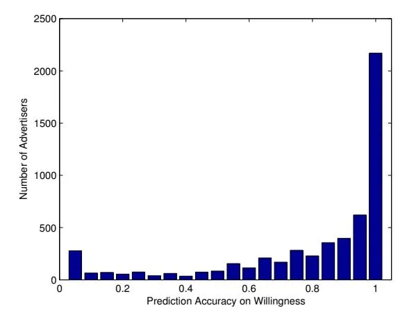
Figure 1: Distribution of the prediction accuracy.

5.2.2 Capability

Second, we investigate the capability function. For this purpose, we set $C_l$ as an identify function, and only consider $W_l$ and $A_l$ . In the capability function $A_l$ , we discretely pick the parameter pair $(\delta_l, N_l)$ from the set $\{0, 0.1, \cdots, 0.9, 1.0\} \times \{0, 1, \cdots, 9, 10\}$ and judge which parameter pair is the best using the data in P2 as described in Section 2.3. We call the advertiser model with the learned willingness and capability functions (without considering the constraint function) Rationality-based Advertiser Behavior model with Willingness and Capability (or RAB-WC for short). Its performance will be reported and discussed in Section 5.3.

5.2.3 Constraint

Third, the constraint function is implemented with a linear regression model trained on P2, using the remaining budget as the feature, according to the discussions in Section 2.4. By applying the constraint function, we get the complete version of the proposed model. We call it Rationality-based Advertiser Behavior model with Willingness, Capability, and Constraint (or RAB-WCC for short). Its performance will be given in Section 5.3.

5.3 Bid Prediction

In this subsection, we compare our proposed advertiser model with six baselines in the task of bid prediction. The predicted bid prices are the direct outputs of the advertiser behavior models. The baselines are listed as follows:

Random Bid Model (RBM) refers to the random method of bid prediction. That is, we will randomly select a bid in the bid strategy space as the prediction.
Most Frequent Model (MFM) refers to an intuitive method for bid prediction, which works as follows. First, we get the

historical bid histogram from the bid values in the training period, and then always output the historically most frequentlyused bid value for the test period. If there are several bid prices that are equally frequently used, we will randomly select one from them.

Best Response Model (BRM) [5] refers to the model that predicts the bid strategy to be the best response by assuming the advertisers know all the competitors’ bids in the previous auction.
Regression Model (RM) [8] refers to the model that predicts the bid strategy using a linear regression function. In our experiments, we used the following 5 features as the input of this function: the average bid change in history, the bid change in the previous time period, click number, remaining budget, and revenue in the previous period.
RAB-WC refers to the model as described in the previous subsection.
RAB-WCC-D refers to the degenerated version of RAB-WCC. That is, we select the bid with the maximum probability in the mixed bid strategy output by RAB-WCC.

We adopt two metrics to evaluate the performances of these advertiser models.

First, we use the likelihood of the test data as the evaluation metric [9]. Specifically, we denote a probabilistic prediction model as $\mathcal{M},^{10}$ which outputs a mixed strategy of advertiser l in period t as $\pi_l^{[t]} = (\pi_{l,0}^{[t]}, \cdots, \pi_{l,B}^{[t]})$ in the bid strategy space $\Omega^0$ . Suppose the index of the real bid strategy of l in period t is $\omega_l^{[t]}$ . Considering a period set $\mathcal{T}$ and an advertiser set $\mathcal{I}$ , we define the following likelihood:

$P_{\mathcal{T},\mathcal{I}}(\mathcal{M}) = \Pi_{t \in \mathcal{T}, l \in \mathcal{I}}(\pi_{l,\omega_i^{[t]}}^{[t]}).$

$P_{\mathcal{T},\mathcal{I}}(\mathcal{M})$ reflects the probability that model $\mathcal{M}$ produces the real data $\omega_l^{[t]}$ for all $t \in \mathcal{T}$ and all $l \in \mathcal{I}$ . To make the metric normalized and positive, we adopt the geometric average and a negative logarithmic function. As a result, we get

$D_{\mathcal{T},\mathcal{I}}(\mathcal{M}) = -\ln(\sqrt{|\mathcal{T}|}\sqrt{P_{\mathcal{T},\mathcal{I}(\mathcal{M})}}) = \frac{-\ln P_{\mathcal{T},\mathcal{I}}(\mathcal{M})}{|\mathcal{T}||\mathcal{I}|}.$

We call it negative logarithmic likelihood (NLL). It can be seen that with the same $\mathcal T$ and $\mathcal I$ , the smaller NLL is, the better prediction $\mathcal M$ gives.

^<sup>10Please note some of the models under investigation are deterministic models. We can still compute the likelihood for them because deterministic models are special cases of probabilistic models.

Second, we use the expected error between the predicted bid strategy and the real bid as the evaluation metric. Specifically, we define the metric as the aggregated expected error (AEE) on a period set T and an advertiser set I, i.e.,

$\sum_{t \in \mathcal{T}} \sum_{l \in \mathcal{I}} \sum_{i=0}^{B} |\pi_{l,i}^{[t]}(b_i - b_{\omega_l^{[t]}})|.$ (3)

The average NLL and AEE on all the 160 queries of the above algorithms are shown in Table 4. We have the following observations from the table.

Our proposed RAB-WCC achieves the best performance compared with all the baseline methods.
RAB-WCC-D performs the second best among these methods, indicating that the bid with the maximum probability in RAB-WCC has been a very good prediction compared with most of the baselines.
RAB-WC performs the third best among these methods, showing that: a) the proposed rationality-based advertiser model can outperform the commonly used algorithms in bid prediction; b) the introduction of the constraint function to the rationality-based advertiser model can further improve its prediction accuracy.
RBM performs almost the worst, which is not surprising due to its uniform randomness.
BRM also performs very bad. Our explanation is as the following. In BRM, we assume the advertisers know all the competitors’ bids before selecting the bids for the next auction. However, the real situation is far from this assumption. So the “best response” will not be the real response for most cases.
MFM model performs better than BRM. This is not difficult to interpret. MFM is a data driven model, without too much unrealistic assumptions. Therefore, it will fit the data better than BRM.
RM performs better than MFM but worse than RAB-WC, RAB-WCC-D, and RAB-WCC. RM is a machine learning model which leverages several features related to the advertiser behaviors, therefore it can outperform MFM which is simply based on counting. However, RM does not consider the rationality levels in its formulation, and therefore it cannot fit the data as well as our proposed model. This indicates the importance of modeling advertiser rationality when predicting their bid strategy changes.

In addition to the average results, we give some example queries and their corresponding NLL and AEE on the 960th auction in P3 in Table 5 and Table 6. The best scores are blackened in the table. At first glance, we see that RAB-WCC achieves the first positions in most of the example queries, while RAB-WCC-D and RAB-WC achieve the first positions for the rest example queries. In most cases, RBM performs the worst, and RM performs moderately.

To sum up, we can conclude that the proposed RAB-WCC method can predict the advertisers’ bid strategies with the best accuracy among all the models under investigation.

5.4 Click and Revenue Prediction

To further test the performance of our model, we apply it to the tasks of click number prediction and revenue prediction.¹¹ We compare our model with two state-of-the-art models on these tasks. The first baseline model is the Structural Model in Sponsored Search [2], abbreviated as SMSS-1. The second baseline model is the Stochastic Model in Sponsored Search [17], abbreviated as SMSS-2. SMSS-1 calculates the expected number of clicks and the expected expenditure for each advertiser by considering some uncertainty assumptions on sponsored search marketplace. SMSS-2 assumes that all the advertisers’ bids are independent and identically distributed and they learn the distribution by mixing all the advertisers’ historical bids.

We use the relative error and absolute error as compared to the real click numbers and revenue in the test period as the evaluation metrics. Specifically, suppose the value output by the model and the ground truth value are φ and ϕ respectively, then the absolute error and the relative error are calculated as |φ − ϕ| and |φ − ϕ|/ϕ respectively. The performance of all the models under investigation are listed in Table 7.

According to the table, we can clearly see that RAB-WCC performs better than both SMSS-1 and SMSS-2. The absolute errors on click number and revenue made by SMSS-1 are very large as compared to the other methods. The relative errors made by SMSS-1 are larger than 50% for both click number and revenue prediction, which are not good enough for practical use. The relative error made by SMSS-2 for revenue prediction is even larger than 80%. In contrast, our proposed RAB-WCC method generates relative errors of no more than 20% for both click and revenue prediction (and the absolute errors are also small). Although the results might need further improvements, a 20% prediction error has already provided quite good references for the search engine to make decision.

Besides the randomized bid strategy and the strategy of selecting the most frequently used bid, there are a number of works on advertiser modeling in the literature. Early work studies some simple cases in sponsored search such as auctions with only two advertisers and auctions in which the advertisers adjust their bids in an alternating manner [1] [21] [18]. Later on, greedy methods were used to model advertiser behaviors. For example, in the random greedy bid strategy [4], an advertiser chooses a bid for the next round of auction that maximizes his/her utility, by assuming that the bids of all the other advertisers in the next round will remain the same as in the previous round. In the locally-envy free bid strategy [10] [16], each advertiser selects the optimal bid price that leads to a certain equilibrium called locally-envy free equilibrium. In [6], the advertiser bid strategies are modeled using the knapsack problem. Competitor-busting greedy bid strategy [22] assumes that an advertiser will bid as high as possible while retaining his/her desired ad slot in order to make the competitors pay as much as possible and thus exhaust their advertising resources. Other similar work includes low-dimensional bid strategy [20], restricted balanced greedy bid strategy [4], and altruistic greedy bid strategy [4]. In [5], a model that predicts the bid strategy to be the best response is proposed by assuming the advertisers know all the competitors’ bids in the previous auction. In [8], a linear regression model is used base on a group of advertiser behavior features. In addition, a bid strategy based on incremental cost per click is discussed in [19]

¹¹After outputting the bid prediction, we simulated the auction process based on those bids and made estimation on the revenue and clicks according to the simulation results.

Table 4: Prediction performance

Model	RBM	MFM	BRM	RM	RAB-WC	RAB-WCC-D	RAB-WCC
NLL	3.939	1.420	2.154	1.289	1.135	1.056	1.018
AEE	35.392	34.748	77.526	40.397	14.616	10.553	8.876

Table 5: Prediction performance on some example queries (NLL)

Model	RBM	MFM	BRM	RM	RAB-WC	RAB-WCC-D	RAB-WCC
car insurance	3.067	1.198	1.777	2.468	0.995	0.975	0.975
disney	2.169	0.541	2.592	0.300	0.130	0.140	0.130
ipad	4.457	1.288	2.075	0.747	0.315	0.325	0.310
jcpenney	2.089	0.511	3.213	0.487	0.263	0.351	0.262
medicare	3.649	1.466	1.750	2.866	1.125	1.127	1.121
stock market	5.068	1.711	2.100	1.839	1.373	1.349	1.362

[2], which proves that an advertiser’s utility is maximized when he/she bids the amount at which his/her value per click equals the incremental cost per click.¹²

However, please note that most of the above works assume that the advertisers have the same rationality and intelligence in choosing the best response to optimize their utilities. Therefore they have significant difference from our work. Actually, to the best of our knowledge, there is no work on advertiser behavior modeling that considers different aspects of advertiser rationality.

7. CONCLUSIONS AND FUTURE WORK

In this work, we have proposed a novel advertiser model which explicitly considers different levels of rationality of an advertiser. We have applied the model to the real data from a commercial search engine and obtained better accuracy than the baseline methods, in bid prediction, click number prediction, and revenue prediction.

As for future work, we plan to work on the following aspects.

First, in Section 2.1, we have assumed that the auctions for different keywords are independent of each other. However, in practice, an advertiser will bid multiple keywords simultaneously and his/her strategies for these keywords may be dependent. We will study this complex setting in the future.
Second, we will study the equilibrium in the auction given the new advertiser model. Most previous work on equilibrium analysis is based on the assumption of advertiser rationality. When we change this foundation, the equilibrium needs to be re-investigated.
Third, we will apply the advertiser model in the function modules in sponsored search, such as bid keyword suggestion, ad selection, and click prediction, to make these modules more robust against the second-order effect caused by the advertiser behavior changes.
Fourth, we will consider the application of the advertiser model in the auction mechanism design. That is, given the advertiser model, we may learn an optimal auction mechanism using a machine learning approach.

APPENDIX

In the appendix, we discuss some properties of the proposed model. Firstly, we give a theorem on the relationship of true value and bid. Secondly, we give a theorem related to the estimation accuracy of the true value.

A. RELATIONSHIP

We discuss about the relationship between true value $v_l$ and our predicted bid strategy. Note that we will mainly focus on the results from the capability function because both willingness and compromise functions are not effected by the true value $v_l$ according to their definitions. For this purpose, by setting $W_l=1$ and $C_l$ as the identity function in $\pi_l$ , we define:

$\boldsymbol{F}(v_l) = E_{\sigma_{\boldsymbol{o}_{-l}}} \left\{ \arg \max_{\boldsymbol{\pi}_l^{(l)}} (\overline{\alpha}_j (v_l - o_{\hat{l}} \overline{s}_{\hat{l}} / \overline{s}_l)) \right\}$

$E(v_l) = (b_1, b_2, ..., b_B)(\mathbf{F}(v_l))^T$

Here $F(v_l)$ is a B-dimension strategy vector and $E(v_l)$ is the average bid of the strategy $F(v_l)$ . Under a very common assumption that ad position effect $\alpha_j$ decreases with the slot index j, Theorem 2 shows that an advertiser with a higher true value will generally set a higher bid to optimize the utility, which is consistent to the intuition. This conclusion shows the consistency of our model in the capability part.

THEOREM 2. Assume $\alpha_j$ decreases in j, then $E(v_l)$ is monotone nondecreasing in $v_l$ .

PROOF. To prove $E(v_l)$ is monotone nondecreasing, we only need to prove that $\forall o_{-l}$ and $\forall \Delta > 0$ ,

$(b_{1}, b_{2}, ..., b_{B}) \left( \underset{\boldsymbol{\pi}_{l}^{(l)}}{\arg \max} (\overline{\alpha}_{j} (v_{l} (1 + \Delta) - o_{\tilde{l}} \overline{s}_{\tilde{l}} / \overline{s}_{l})) \right)$

$\geq (b_{1}, b_{2}, ..., b_{B}) \left( \underset{\boldsymbol{\pi}_{l}^{(l)}}{\arg \max} (\overline{\alpha}_{j} (v_{l} - o_{\tilde{l}} \overline{s}_{\tilde{l}} / \overline{s}_{l})) \right), \tag{4}$

and then the ” $\geq$ ” will keep unchanged in the expectation of $o_{-l}$ . We denote $j^{\Delta}$ and $j^0$ as the best rank of l for the cases that true values are $v_l(1+\Delta)$ and $v_l$ respectively. Here $o_{-l}$ is fixed and “best rank” means the rank that leads to the optimal utility.

^<sup>12Incremental cost per click is defined as the advertiser’s average cost of additional clicks received at a better ad slot.

Table 6: Prediction performance on some example queries (AEE)

Model	RBM	MFM	BRM	RM	RAB-WC	RAB-WCC-D	RAB-WCC
car insurance	89.459	89.883	305.703	107.335	33.207	22.188	12.760
disney	5.019	4.895	9.703	0.217	0.297	0.171	0.140
ipad	16.355	15.428	30.856	0.662	0.975	0.458	0.385
jcpenney	5.036	5.145	16.337	1.476	1.411	1.165	0.209
medicare	98.206	99.014	225.774	111.248	20.221	16.695	3.744
stock market	37.576	38.360	72.640	97.035	5.824	4.137	1.486

We denote $\hat{l}_{\Delta}$ and $\hat{l}_{0}$ as the advertisers who rank at $(j^{\Delta}+1)$ and $(j^{0}+1)$ respectively. Note that for a fixed $o_{-l}$ , $j^{\Delta}$ and $j^{0}$ can be different due to different true value of l. If we are able to prove $j^{\Delta} \geq j^{0}$ , then the inequality (4) will be valid since a nondecreasing best ranking yields a nondecreasing best bid strategy.

As $j^0$ is the best rank for the true value $v_l$ , we have

$\overline{\alpha}_{j^0}(v_l - o_{\hat{l}_0} \overline{s}_{\hat{l}_0} / \overline{s}_l) \ge \overline{\alpha}_{j^{\Delta}}(v_l - o_{\hat{l}_{\Lambda}} \overline{s}_{\hat{l}_{\Lambda}} / \overline{s}_l). \tag{5}$

Assuming $j^{\Delta} < j^0$ , we have,

$\overline{\alpha}_{j^0} v_l \Delta > \overline{\alpha}_{j^{\Delta}} v_l \Delta. \tag{6}$

By adding (3) and (4), we got,

$\overline{\alpha}_{j^0}(v_l(1+\Delta) - o_{\hat{l}_0}\overline{s}_{\hat{l}_0}/\overline{s}_l) > \overline{\alpha}_{j^\Delta}(v_l(1+\Delta) - o_{\hat{l}_\Lambda}\overline{s}_{\hat{l}_\Lambda}/\overline{s}_l).$

This equation reveals that $j^0$ is a better rank than $j^{\Delta}$ and $j^{\Delta}$ should not be the best rank for the true value $v_l(1 + \Delta)$ , which is contradictive to the definition of $j^{\Delta}$ . Therefore, the assumption $j^{\Delta} < \underline{j^0}$ is not valid, which also finishes our proof of this theo-

В. ESTIMATION ACCURACY

As discussed in Section 4, we choose the model in [9] for the true value prediction. Usually, the estimation is not perfect and there might be some errors. Fortunately, we can prove a theorem which guarantees that the solution of this model will keep accurate if the estimation errors are not very large. This holds true because the payment rule of GSP is discrete and it allows the small-scale vibration of true value.

Before introducing the theorem, we give some notations first. For a fixed $o_{-l}$ and true value $v_l$ , l’s best rank is denoted as $BR_{o_{-l}}$ (Best Rank), the optimal utility is denoted as $BU_{o_{-1}}$ , and the ranking score of $\hat{l}$ (the one ranked next to l) in the optimal case is denoted $BS_{o_{-1}}$ . To describe the theorem, we also denote the second optimal utility as $SU_{o_{-l}}$ (Second Utility), which is the largest utility less than $BU_{o_{-1}}$ in the fixed $o_{-1}$ .

Theorem 3. We assume that $\alpha_j$ decreases in j and set $\theta = \max_{o_{-l}}(\frac{SU_{o_{-l}}}{BU_{o_{-l}}})$ , $\rho = \max_{o_{-l}}(BR_{o_{-l}})$ , and $\omega = \max_{o_{-l}}(BS_{o_{-l}})$ , $(v_l - \omega/\overline{s}_l > 0)$ . Let $v_l$ increase by $\Delta v_l$ $(\Delta \in R)$ , then $F(v_l)$ will keep unchanged if $|\Delta| \leq \frac{\alpha_{\rho}}{\alpha_{1}}(1-\theta)(1-\frac{\omega}{\overline{s}_{l}v_{l}})$ , where $\alpha_{1}$ is the CTR at the first position.

In order to prove the bound of $\Delta$ keeps $F(v_l)$ unchanging, we prove the following lemma instead.

Lemma 1. If $\Delta$ satisfies $|\Delta| \leq \frac{\alpha_{\rho}}{\alpha_{1}}(1-\theta)(1-\frac{\omega}{\overline{s}_{l}v_{l}})$ , then $\forall o_{-l}$ we have, $argmax_{\pi_{l}^{(l)}}\overline{\alpha}_{j}(v_{l}(1+\Delta)-o_{l}\overline{s}_{l}/\overline{s}_{l}) = argmax_{\pi_{l}^{(l)}}\overline{\alpha}_{j}(v_{l}-c_{l})$

The proof of Theorem 3 will be finished at once after we sum up all the cases of $o_{-l}$ in Lemma 1.

Table 7: Prediction performance in applications

SMSS-1	SMSS-2	RAB-WCC
0.52	0.11	0.19
2.02	0.71	0.23
0.54	0.83	0.18
659.06	124.80	25.75
	0.52 2.02 0.54	0.52 0.11 2.02 0.71 0.54 0.83

PROOF. Since a change of ” $argmax_{\pi^{(l)}}$ ” is equivalent to a change of ” $BR_{o_{-1}}$ ”, we consider the critical point that the increase of $\Delta$ makes the best rank transfer exactly from $j^0$ to $j^\Delta$ ( $j^0 \neq j^\Delta$ ). Thus we have: $\exists j^\Delta(j^\Delta \neq j^0), s.t.\ j^\Delta, j^0$ maximizes $\overline{\alpha}_j(v_l(1+$

$\Delta$ ) – $o_i \bar{s}_i / \bar{s}_l$ ) simultaneously, and then we can get,

$\overline{\alpha}_{j^{\Delta}}(v_l(1+\Delta) - o_{\hat{l}_{\Delta}}\overline{s}_{\hat{l}_{\Delta}}/\overline{s}_l) = \overline{\alpha}_{j^0}(v_l(1+\Delta) - o_{\hat{l}_0}\overline{s}_{\hat{l}_0}/\overline{s}_l). \tag{7}$

From equation (7) we have

$\Delta = \frac{\overline{\alpha}_{j^0} (v_l - o_{\hat{l}_0} \overline{s}_{\hat{l}_0} / \overline{s}_l) - \overline{\alpha}_{j^{\Delta}} (v_l - o_{\hat{l}_{\Delta}} \overline{s}_{\hat{l}_{\Delta}} / \overline{s}_l)}{v_l (\alpha_{j^{\Delta}} - \alpha_{j^0})}.$ (8)

Assume there is a $\theta_0$ such that

$\overline{\alpha}_{j\Delta}(v_l - o_{\hat{l}_{\Delta}}\overline{s}_{\hat{l}_{\Delta}}/\overline{s}_l) = \theta_0 \overline{\alpha}_{j0}(v_l - o_{\hat{l}_0}\overline{s}_{\hat{l}_0}/\overline{s}_l). \tag{9}$

Then equation (8) is transformed as,

$\Delta = \frac{(1 - \theta_0)\overline{\alpha}_{j^0}(v_l - o_{\hat{l}_0}\overline{s}_{\hat{l}_0}/\overline{s}_l)}{v_l(\alpha_{j^\Delta} - \alpha_{j^0})}$

$= (1 - \theta_0)\frac{\alpha_{j^0}}{\alpha_{j\Delta} - \alpha_{j^0}}(1 - \frac{o_{\hat{l}_0}\overline{s}_{\hat{l}_0}/\overline{s}_l}{v_l}). \quad (10)$

Considering $j^0$ is the best rank, from equation (9) we have,

$\theta_0 = \frac{\overline{\alpha}_{j\Delta} (v_l - o_{\hat{l}_{\Delta}} \overline{s}_{\hat{l}_{\Delta}} / \overline{s}_l)}{\overline{\alpha}_{j0} (v_l - o_{\hat{l}_0} \overline{s}_{\hat{l}_0} / \overline{s}_l)} \le \frac{SU_{o_{-l}}}{BU_{o_{-l}}} \le \theta < 1.$ (11)

In addition, there holds

$j^{0} \leq \max_{\boldsymbol{\sigma}_{-l}}(BR_{\boldsymbol{\sigma}_{-l}}) = \rho,$

$\alpha_{j^{0}} \geq \alpha_{\rho}, \left|\frac{\alpha_{j^{0}}}{\alpha_{j^{\Delta}} - \alpha_{j^{0}}}\right| > \frac{\alpha_{\rho}}{\alpha_{1}},$ (12)

$o_{\hat{l}_0} \overline{s}_{\hat{l}_0} = BS_{o_{-l}} \le max_{o_{-l}} (BS_{o_{-l}}) = \omega.$ (13)

According to (10) and (11),(12),(13), we finally have,

$|\Delta| = |1 - \theta_0| \frac{\alpha_{j^0}}{|\alpha_{j^{\Delta}} - \alpha_{j^0}|} (1 - \frac{o_{\hat{l}_0} \overline{s}_{\hat{l}_0}}{\overline{s}_l v_l}) > \frac{\alpha_{\rho}}{\alpha_1} (1 - \theta) (1 - \frac{\omega}{\overline{s}_l v_l}).$

As $\Delta$ is the critical point, for any fixed $o_{-l}$ , if $|\Delta| \leq \frac{\alpha_{\rho}}{\alpha_{1}}(1 \theta)(1- rac{\omega}{\overline{s}_lv_l}),~BR_{m{o}_{-l}}$ and ” $argmax_{\pi_l^{(l)}}$ ""will keep unchanged. This ends our proof of Lemma 1.

C. REFERENCES

[1] K. Asdemir. Bidding patterns in search engine auctions. In Second Workshop on Sponsored Search Auctions (2006), ACM Electronic Commerce. Press., 2006.
[2] S. Athey and D. Nekipelov. A structural model of sponsored search advertising auctions., 2010. Available at http://groups.haas.berkeley.edu/ marketing/sics/pdf_2010/paper_athey.pdf.
[3] A. Broder, E. Gabrilovich, V. Josifovski, G. Mavromatis, and A. Smola. Bid generation for advanced match in sponsored search. In Proceedings of the fourth ACM international conference on Web search and data mining, WSDM ‘11, pages 515–524, New York, NY, USA, 2011. ACM.
[4] M. Cary, A. Das, B. Edelman, I. Giotis, K. Heimerl, A. R. Karlin, C. Mathieu, and M. Schwarz. Greedy bidding strategies for keyword auctions. In EC ‘07 Proceedings of the 8th ACM conference on Electronic commerce. ACM Press., 2007.
[5] M. Cary, A. Das, B. G. Edelman, I. Giotis, K. Heimerl, A. R. Karlin, C. Mathieu, and M. Schwarz. On best-response bidding in gsp auctions., 2008. Available at http: //www.hbs.edu/research/pdf/08-056.pdf.
[6] D. Chakrabarty, Y. Zhou, and R. Lukose. Budget constrained bidding in keyword auctions and online knapsack problems. In WWW ‘07 Proceedings of the 16th international conference on World Wide Web. ACM Press., 2007.
[7] Y. Chen, G.-R. Xue, and Y. Yu. Advertising keyword suggestion based on concept hierarchy. In WSDM ‘08 Proceedings of the international conference on Web search and web data mining. ACM Press., 2008.
[8] Y. Cui, R. Zhang, W. Li, and J. Mao. Bid landscape forecasting in online ad exchange marketplace. In KDD ‘11 Proceedings of the 17th ACM SIGKDD international conference on Knowledge discovery and data mining. ACM Press., 2011.
[9] Q. Duong and S. Lahaie. Discrete choice models of bidder behavior in sponsored search. In Workshop on Internet and Network Economics (WINE). Press., 2011.
[10] B. Edelman, M. Ostrovsky, and M. Schwarz. Internet advertising and the generalized second-price auction: Selling billions of dollars worth of keywords. In The American Economic Review., 2007.
[11] T. Graepel, J. Q. Candela, T. Borchert, and R. Herbrich. Web-scale bayesian click-through rate prediction for sponsored search advertising in microsoft’s bing search engine. In Proceedings of the 27th International Conference on Machine Learning. ACM, 2010.
[12] J. C. Harsanyi. Games with incomplete information played by bayesian players, i-iii. In Management Science., 1967/1968.
[13] J. Jansen. Understanding Sponsored Search: Core Elements of Keyword Advertising. Cambridge University Press., 2011.
[14] B. Kitts and B. Leblanc. Optimal bidding on keyword auctions. In Electronic Markets. Routledge Press., 2004.
[15] D. C. Liu and J. Nocedal. On the limited memory bfgs method for large scale optimization. In Journal of Mathematical Programming. Springer-Verlag New York., 1989.
[16] C. Nittala and Y. Narahari. Optimal equilibrium bidding strategies for budget constrained bidders in sponsored search auctions. In Operational Research: An International Journal. Springer Press, 2011.
[17] F. Pin and P. Key. Stochasitic variability in sponsored search auctions: Observations and models. In EC ‘11 Proceedings of the 12th ACM conference on Electronic commerce. ACM Press., 2011.
[18] S. S. S. Reddy and Y. Narahari. Bidding dynamics of rational advertisers in sponsored search auctions on the web. In Proceedings of the International Conference on Advances in Control and Optimization of Dynamical Systems. Press., 2007.
[19] H. R. Varian. Position auctions. In International Journal of Industrial Organization, 2006.
[20] Y. Vorobeychik. Simulation-based game theoretic analysis of keyword auctions with low-dimensional bidding strategies. In UAI ‘09 Proceedings of the Twenty-Fifth Conference on Uncertainty in Artificial Intelligence. AUAI Press., 2009.
[21] X. Zhang and J. Feng. Finding edgeworth cycles in online advertising auctions. In Proceedings of the 26th International Conference on Information Systems ICIS. Press., 2006.
[22] Y. Zhou and R. Lukose. Vindictive bidding in keyword auctions. In ICEC ‘07 Proceedings of the ninth international conference on Electronic commerce. ACM Press., 2007.