To Broad Match Or Not To Broad Match An Auctioneers Dilemma

Abstract

We initiate the study of an interesting aspect of sponsored search advertising, namely the consequences of broad match- a feature where an ad of an advertiser can be mapped to a broader range of relevant queries, and not necessarily to the particular keyword(s) that ad is associated with. In spite of its unanimously believed importance, this aspect has not been formally studied yet, perhaps because of the inherent difficulty involved in formulating a tractable framework that can yield meaningful conclusions. In this paper, we provide a natural and reasonable framework that allows us to make definite statements about the economic outcomes of broad match.

Starting with a very natural setting for strategies available to the advertisers, and via a careful look through the algorithmic lens, we first propose solution concepts for the game originating from the strategic behavior of advertisers as they try to optimize their budget allocation across various keywords.

Next, we consider two broad match scenarios based on factors such as information asymmetry between advertisers and the auctioneer (i.e. the search engine company), and the extent of auctioneer’s control on the budget splitting. In the first scenario, the advertisers have the full information about broad match and relevant parameters, and can reapportion their own budgets to utilize the extra information; in particular, the auctioneer has no direct control over budget splitting. We show that, the same broad match may lead to different equilibria, one leading to a revenue improvement, whereas another to a revenue loss. This leaves the auctioneer in a dilemma - whether to broad-match or not, and consequently leaves him with a computational problem of predicting which broad matches will provably lead to revenue improvement. This motivates us to consider another broad match scenario, where the advertisers have information only about the current scenario, i.e., without any broad-match, and the allocation of the budgets unspent in the current scenario is in the control of the auctioneer. Perhaps not surprisingly, we observe that if the quality of broad match is good, the auctioneer can always improve his revenue by judiciously using broad match. Thus, information seems to be a double-edged sword for the auctioneer. Further, we also discuss the effect of both broad match scenarios on social welfare.

1 Introduction and Motivation

The importance of understanding the various aspects of sponsored search advertising(SSA) is now well known. Indeed, this advertising framework has been studied extensively in recent years from algorithmic[12, 6, 13, 18], game-theoretic[5, 22, 1, 9, 3, 4, 11], learning-theoretic[7, 24, 19] perspectives, as well as, from the viewpoint of emerging diversification in the internet economy[20, 21]. Specifically, among others, these studies include important aspects such as (i) the design of mechanisms for optimizing the revenue of the auctioneer, (ii) budget optimization problem of an advertiser, (iii) analyzing the bidding behavior of advertisers in the auction of a keyword query, (iv) learning the Click-Through-Rates and (v) the role of for-profit mediators. In the present paper, our goal is to initiate the study of yet another interesting aspect of SSA, namely the consequences of broad match. Despite its unanimously believed importance, to the best of our knowledge, this aspect has not been formally studied yet, probably because of the hardness in employing a proper framework for such an study. Our main aim in this paper is to attempt to provide such a framework. In the rest part of this section, we start by an informal introduction to broad match, then while establishing the need of a framework to study broad match we provide a glimpse of the present work.

1.1 What is Broad Match?

In SSA format, each advertiser has a set of keywords relevant to her products and a daily budget that she wants to spend on these keywords. Further, for each of these keywords she has a true value associated with it that she derives when a user clicks on her ad corresponding to that keyword, and based on this true value she reports her bid to the search engine company (i.e. the auctioneer) to indicate the maximum amount she is willing to pay for a click. When a user queries for a keyword, the auctioneer runs an auction among all the advertisers interested in that keyword whose budget is not over yet. The advertisers winning in this auction are allocated an ad slot each, determined according to the auction’s allocation rule and an advertiser is charged, whenever the user clicks on her ad, an amount determined according to the auction’s payment rule. In this way, for each of the advertisers, each of her ads is matched to queries of the particular keyword(s) that ad is associated with.

Broad Match is a feature where an ad of an advertiser can be mapped to a broader range of relevant queries, and not necessarily to the particular keyword(s) that ad is associated with. Such relevant queries could be possible variations of the associated keyword or could even correspond to a completely different keyword which is conceptually related to the associated keyword. For example, the variations of keyword “Scuba” could include “Scuba diving”, “Scuba gear”, “Scuba shops in Los Angeles” etc and conceptually related keywords could include “Snorkeling”, “under water photography” etc. Similarly, for the keyword “internet advertising”, the variations could include “banner advertising”, “PPC advertising”, “advertising on the internet”, “keyword advertising”, “online advertising” etc, and conceptually related keywords could include “adword”, “adsense” etc; for the keyword “horse race”, the variations could include “horse racing tickets”, “horse race betting”, “online horse racing” etc, and a conceptually related keyword could be “thoroughbred”.

1.2 The Need of a Framework to Study Broad Match

To study the effect of incorporating broad match on macroscopic quantities such as revenue of the auctioneer, social value etc, compared to the scenario without broad match, we must consider the interaction among various keywords. We must take into account the changes in the bidding behavior of advertisers for specific keyword queries, as well as, the effect of changes in their budget allocation across various keywords. As we mentioned earlier, the incentive properties of query specific keyword auction is well analyzed in articles such as[5, 22, 1, 9, 3, 4, 11]. Further, the budget optimization problem of an advertiser, that is to spend the budget across various keywords in an optimal manner given quantities such as keyword specific costper-clicks, expected number of clicks, and payoffs as a function of bid, has also been studied under various models[6, 13, 18]. However, the incentive constraints originating from such budget optimizing strategic behavior of advertisers has not been formally studied yet. In particular, there is no proposed solution concept pertinent for predicting the stable behavior of advertisers in this game[2]. On the other hand, for the analysis of the effect of incorporating broad match, it becomes inevitable to have such a solution concept, that is a notion of equilibrium behavior, under which we can compare the quantities such as revenue of the

auctioneer, social value etc, for the two scenarios one with the broad match and the one without it at their respective equilibrium points.

1.3 Our Results

Our first goal in this paper is to attempt to provide a reasonable solution concept for the game originating from the strategic behavior of advertisers as they try to optimize their budget allocation/splitting across various keywords. We realize that without some reasonable restrictions on the set of available strategies to the advertisers, it is a much harder task to achieve[2]. To this end, we consider a very natural setting for available strategies- (i) first split/allocate the budget across various keywords and then (ii) play the keyword query specific bidding/auction game as long as you have budget left over for that keyword when that query arrives -thereby dividing the overall game in to two stages. In the spirit of [5, 22] wherein the query specific keyword auction is modeled as a static one shot game of complete information despite its repeated nature in practice, we model the budget splitting too as a static one shot game of complete information because if the budget splitting and bidding process ever stabilize, advertisers will be playing static best responses to their competitors’ strategies.

Now, with this one shot complete information game modeling, the most natural solution concept to consider is pure Nash equilibrium. However, in our case, it seems to be a very strong notion of equilibrium behavior if we look through our algorithmic glasses1 because, as we argue in the paper, an advertiser’s problem of choosing her best response is computationally hard. Consequently, we first consider a weaker solution concept based on local Nash equilibrium. We show that there is a strongly polynomial time (polynomial in number of advertisers, keywords and ad slots and not the volume of queries or total daily budget) algorithm to compute an advertiser’s locally best response. This notion of equilibrium, which we call broad match equilibrium (BME), is defined in terms of marginal payoff (or bang-per-buck) for various keywords corresponding to a budget splitting, and looks similar to the definition of user equilibrium/Waldrop equilibrium in routing and transportation science literature[17]. Further, there is a strongly poly-time algorithm to compute an advertiser’s approximate best response as well. Therefore, the approximate Nash equilibrium (ǫ-NE) is also reasonable in our setting. Indeed, all the conclusions of our work hold true irrespective of which of these two solution concepts we adopt, the BME or the ǫ*-NE*.

In the full information setting, under the solution concept of BME we obtain several observations by explicitly constructing examples. In particular, even with this natural and reasonably restricted notion of stable behavior, we observe that same broad match might lead to different BMEs where one BME might lead to an improvement in the revenue of the auctioneer over the scenario without broad match while the other to a loss in revenue, even when the quality of broad-match is very good. This leaves the auctioneer in a dilemma about whether he should broad-match or not. If he could somehow predict which choice of broad match lead to a revenue improvement for him and which not, he could potentially choose the ones leading to a revenue improvement. Further, the same examples imply the same conclusions under the solution concept of ǫ*-NE*. This brings forth one of the big questions left open in this paper, that is of efficiently computing a BME / ǫ*-NE*, if one exists, given a choice of broad match.

Note that in the above scenario of broad match, the advertisers had all the relevant information about the broad match, and the control of budget splitting is in the hands of respective advertisers. We also explore another broad match scenario where the advertisers have information only about the scenario without broadmatch, and they allow the auctioneer to spend their excess budgets (i.e the budget unspent in the scenario without broad match), in whatever way the auctioneer wants, in the hope of potential improvements in their payoffs. Perhaps not surprisingly, we observe that if the quality of broad match is good, the auctioneer

¹Efficient computability is an important modeling prerequisite for solution concepts. In the words of Kamal Jain, “If your laptop cannot find it, neither can the market”[14].

can always improve his revenue. Thus, information seems to be a double-edged sword for the auctioneer. Further, we also discuss the effect of both broad match scenarios on social welfare.

1.4 Organization of the Paper

Rest of the paper is organized as follows. In Section 2, we describe the formal setting of the query specific keyword auctions. In Section 3, we define Broad Match Graph, a weighted bipartite graph between the set of advertisers and the set of keywords, which serves as the basic back bone in terms of which we formulate all our notions and results. In Section 4, we present the defining characteristics of the two broad match scenarios studied in this paper, in terms of factors such as information asymmetry and the extent of auctioneer’s control on the budget splitting. The Section 5 is devoted to the study of broad match scenario in the full information setting where the auctioneer has no direct control on the budget splitting. This is essentially the most contributing part of this paper wherein first we appropriately model the game originating from the strategic behavior of advertisers as they try to optimize their budget allocation/splitting across various keywords, then we propose appropriate solution concepts for this game, and finally study the effect of broad match under this proposed framework. In Section 6, we study the other broad match scenario, where advertisers do not have full information about the broad match being performed and the auctioneer partially controls the budget splitting. Finally, in Section 7, we conclude with potential directions for future work motivated by the present paper.

2 Keyword Auctions

There are K slots to be allocated among N ( $\geq K$ ) bidders (i.e. the advertisers). A bidder i has a true valuation $v_i$ (known only to the bidder i) for the specific keyword and she bids $b_i$ . The expected click through rate (CTR) of an ad put by bidder i when allocated slot j has the form $CTR_{i,j} = \gamma_j e_i$ i.e. separable in to a position effect and an advertiser effect. $\gamma_j$ ’s can be interpreted as the probability that an ad will be noticed when put in slot j and it is assumed that $\gamma_j > \gamma_{j+1}$ for all $1 \leq j \leq K$ and $\gamma_j = 0$ for j > K. $e_i$ can be interpreted as the probability that an ad put by bidder i will be clicked on if noticed and is referred to as the relevance of bidder i. The payoff/utility of bidder i when given slot j at a price of p per-click is given by $e_i\gamma_j(v_i-p)$ and they are assumed to be rational agents trying to maximize their payoffs.

As of now, Google as well as Yahoo! use schemes closely modeled as RBR(rank by revenue) with GSP(generalized second pricing). The bidders are ranked in the decreasing order of $e_ib_i$ and the slots are allocated as per this ranks. For simplicity of notation, assume that the ith bidder is the one allocated slot i according to this ranking rule, then i is charged an amount equal to $\frac{e_{i+1}b_{i+1}}{e_i}$ per-click. This mechanism has been extensively studied in recent years[5, 9, 22, 11]. The solution concept that is widely adopted to study this auction game is a refinement of Nash equilibrium independently proposed by Varian[22] and Edelman et al[5]. Under this refinement, the bidders have no incentive to change to another positions even at the current price paid by the bidders currently at that position. Edelmen et al [5] calls it locally emy-free equilibria and argue that such an equilibrium arises if agents are raising their bids to increase the payments of those above them, a practice which is believed to be common in actual keyword auctions. Varian[22] called it symmetric Nash equilibria(SNE) and provided some empirical evidence that the Google bid data agrees well with the SNE bid profile. In particular, an SNE bid profile $b_i$ ‘s satisfy

$(\gamma_i - \gamma_{i+1})v_{i+1}e_{i+1} + \gamma_{i+1}e_{i+2}b_{i+2} \le \gamma_i e_{i+1}b_{i+1} \le (\gamma_i - \gamma_{i+1})v_i e_i + \gamma_{i+1}e_{i+2}b_{i+2}$ (1)

for all $i=1,2,\ldots,N$ . Now, recall that in the RBR with GSP mechanism, the bidder i pays an amount $\frac{e_{i+1}b_{i+1}}{e_i}$ per-click, therefore the expected payment i makes per-impression is $\gamma_i e_i \frac{e_{i+1}b_{i+1}}{e_i} = \gamma_i e_{i+1}b_{i+1}$ .

Thus the best SNE bid profile for advertisers (worst for the auctioneer) is minimum bid profile possible according to Equation 1 and is given by

$\gamma_i e_{i+1} b_{i+1} = \sum_{j=i}^{K} (\gamma_j - \gamma_{j+1}) v_{j+1} e_{j+1}$ (2)

and therefore, the revenue of the auctioneer at this minimum SNE is

$\sum_{i=1}^{K} \gamma_{i} e_{i+1} b_{i+1} = \sum_{i=1}^{K} \sum_{j=i}^{K} (\gamma_{j} - \gamma_{j+1}) v_{j+1} e_{j+1}$

$= \sum_{i=1}^{K} (\gamma_{j} - \gamma_{j+1}) j v_{j+1} e_{j+1}.$ (3)

3 Broad Match Graph

In this section, we set up a basic backbone to study the dynamics of bidding across various related keywords, in the sponsored search advertising, via a bipartite graph between the set of bidders (i.e. the advertisers) and the set of keywords with the parameters $(N, M, K, S = (s_{i,j}), B = (B_i), V = (V_j))$ as follows.

• Keywords: M is the number of keywords in consideration. We will denote the set of keywords $\{1, 2, ..., M\}$ by M. Further, $V_j$ is the total (expected) volume of queries for the keyword j for a given period of time which we call a “day”. These may not be all the keywords a particular advertiser may be interested in bidding on but one of the sets of keywords which are related by some category/concept that the advertiser is interested in bidding on e.g. for selling the same product or service.
• Bidders/Advertisers: N is the total number of bidders interested in the above M keywords. We will denote the set of bidders $\{1, 2, \ldots, N\}$ by $\mathbb{N}$ . Further, $B_i$ is the total budget of the bidder i for a “day” that she wants to spend on these keywords.
• Slots: K is the maximum number of ad-slots available. Let L be the number of advertisers with sufficient budgets when a particular query of a keyword j arrives then for that query of j, the slot-clickability (i.e. the position based CTRs) are defined to be $\gamma_l$ corresponding to a slot l for $l \leq \min\{K, L\}$ and zero otherwise².
• Valuation Matrix: Let $v_{i,j}$ be the true value of the bidder i for the keyword j and $e_{i,j}$ be her $relevance^2$ (quality score) for j. We call the $N \times M$ matrix S, with (i,j)th entries defined as $s_{i,j} = v_{i,j}e_{i,j}$ , as the $valuation\ matrix$ . For a keyword j for which a bidder i has no interest or is not allowed to bid, $s_{i,j} := -\infty$ . In the revenue/efficiency/payoffs calculations at SNE, it is enough to know $s_{i,j}$ and not the $v_{i,j}$ and $e_{i,j}$ separately, therefore, in this paper we will often refer only to $s_{i,j}$ and not $v_{i,j}$ and $e_{i,j}$ individually.
• Broad Match Graph (BMG): Given instance parameters (N, M, K, S, B, V), a bipartite graph $G = (\mathcal{N}, \mathcal{M}, \mathcal{E})$ , with vertex sets $\mathcal{N}$ and $\mathcal{M}$ and edge set $\mathcal{E} = \{(i, j) : i \in \mathcal{N}, j \in \mathcal{M}, s_{i,j} > 0\}$ , is constructed. Further, each edge $(i, j) \in \mathcal{E}$ is associated with a weight $s_{i,j}$ . The weight of a node $i \in \mathcal{N}$ is $B_i$ and that of a node $j \in \mathcal{M}$ is $V_j$ . Furthermore, an $i \in \mathcal{N}$ will be called an ad-node and an $j \in \mathcal{M}$ will be referred to as a keyword-node.

^<sup>2We assume that the clicks-through-rates(CTRs) are separable.

• Extension of a BMG: A BMG $G' = (\mathcal{N}, \mathcal{M}, \mathcal{E}')$ for the instance (N, M, K, S’, B, V) is called an extension of a BMG $G = (\mathcal{N}, \mathcal{M}, \mathcal{E})$ for the instance (N, M, K, S, B, V) if $\mathcal{E} \subset \mathcal{E}'$ and $s'_{i,j} = s_{i,j}$ for all $(i,j) \in \mathcal{E}$ . Interpretation is that the instance represented by an extension is more broader in the sense that an advertiser has a choice to be and could be matched to a larger set of keywords. Indeed, we will formally refer an extension $G' = (\mathcal{N}, \mathcal{M}, \mathcal{E}')$ to be a broad-match for its base $G = (\mathcal{N}, \mathcal{M}, \mathcal{E})$ . Note that, without loss of generality, this definition of extension (broad-match) captures the possibility that new keywords are introduced. This is because we can always think that a new keyword to be included was already there as an isolated node and now we are creating only edges.

4 Information Asymmetry, Budget Splitting and Two Broad Match Scenarios

Depending on how much information the auctioneer (i.e. the search engine company) provides to advertisers about various parameters, such as CTRs, conversion rates, volume of queries etc, related to the keywords and depending on who splits the daily budget across the various keywords, the auctioneer or the advertisers, we consider the following two scenarios for broad matching:

• I) AdBM: Advertisers Controlled Broad Match, extra information to advertisers, advertisers split their budgets.
• II) AcBM: Auctioneer Controlled Broad Match, no extra information to advertisers, auctioneer splits the budget.

Formally, let $G' = (\mathcal{N}, \mathcal{M}, \mathcal{E}')$ be the broad-match for $G = (\mathcal{N}, \mathcal{M}, \mathcal{E})$ , then we characterize these two scenarios of broad-match based on the following factors(ref. Table 1):

• Information asymmetry: Of course, advertisers already have all the information about the BMG G. That is, they all know their CTRs, conversion rates, volume of queries, who participates how long, spends and bids how much on which keyword, across various keywords they are bidding currently. It is the knowledge about these quantities for the part of the extension G’ which is not in G i.e. along the edges in $\mathcal{E}' \setminus \mathcal{E}$ that advertisers may or may not be aware of depending on whether the auctioneer provides this information to them or not³. In AcBM scenario, advertisers do not have this information. At most what they know is that there is some broad-match the auctioneer is performing and they can effect the dynamics on the extension G’ only passively through their bidding behavior on $G^4$ . In AdBM scenario, there is no such asymmetry in information. Advertisers know (or are rather informed by the auctioneer) all the information about $\mathcal{E}' \setminus \mathcal{E}$ .
• Extent of auctioneer’s control on the budget splitting: In AdBM scenario, the auctioneer has no control over the budget splitting. It is upto the advertisers to decide which keywords they want to participate in and how much budget they want to spend on each of those keywords. Thus, the budget splitting of an advertiser, across various keywords she is connected to in G’, is in her own control and she can split her budget so as to maximize her total payoff across those keywords. As discussed in section 1.2, this brings in another layer of incentive constraints from advertisers besides choosing

^<sup>3Of course, to learn these relevance scores there might be a cost incurred by the auctioneer in the short run, nevertheless if the broad-match quality is good, this cost will generally be minimal.

^<sup>4As we know, in the sponsored search advertising, advertisers effectively derive their valuations from the rate of conversion which might very well change by broad match and accordingly bidders may adjust their true values (and consequently the bids) due to broad match. This might lead to another level of cost to the auctioneer due to uncertainty in performing broad-match. Nevertheless, if the broad-match quality is good, this cost will generally be minimal.

	AdBM	AcBM
Information asymmetry	No	Yes
	(advertisers know all info on new edges)	(advertisers don’t know info on new edges)
Extent of auctioneer’s control on the budget splitting	No Control	Limited Control
		(only for the excess budgets)
An advertiser’s starting time for a keyword	Very First Query	Any Query
		(only for the part auctioneer controls)

Table 1: Two Broad-Match Scenarios

the bid values for individual queries. In AcBM scenario, the auctioneer does have some control over budget splitting. At one extreme, an advertiser might give the complete control to the auctioneer for splitting her budget across various keywords letting the auctioneer decide how much should be spent on which keyword. In this case, since the control will be completely in the hands of the auctioneer it can perform the budget splitting so as to maximize his own total revenue without much concern to the welfare of advertisers. Therefore, advertisers would hardly give such a full control to the auctioneer. However, it is reasonable that an advertiser allows the auctioneer to spend her excess budget i.e. the budget unspent in the case of G, in whatever way the auctioneer wants to spend it in G ′ , in hope of an additional payoff. Note that there must be some advertisers with excess budget for the AcBM to make sense. If every advertiser is already spending its all budget then why to take all the pain of doing a broad-match5 . In our study of AcBM in Section 6, we consider this limited control setting. Another issue the auctioneer faces in AcBM is that what bid profiles to use along the edges in E \ E. The auctioneer must perform these calculations in a manner to maintain equilibrium across the keywords meaning that the advertisers should not be indirectly compelled to revise their true values along the edges in G⁴ . This assumption is reasonable as at SNE the auctioneer can estimate the true values from the equilibrium bids on G and then along with the new information gathered for E ′ \ E, can do the proper SNE bids calculations on the behalf of the advertisers.

• An advertiser’s starting time for a keyword: In AdBM scenario, an advertisers participates in all keywords she is interested in starting with its first query until her budget allocated for that keyword is spent or there are no more queries for that keyword6 . In AcBM scenario, however, since the auctioneer is controlling at least a part of the budget splitting, and unlike advertisers, since it can easily track what happens at which query in an online manner, it can choose to bring in an advertiser’s budget along an edge starting with any particular query of that keyword. For example, it can bring advertiser i in the auction of keyword j starting at say 1000th query of j.

Now, let us illustrate the above two scenarios via an example by considering the BMG given in Figure 1 (i.e. the graph without the edge (3, 1)) and its extension given in the same figure (i.e. the graph including the edge (3, 1)). Further, each query is sold via a GSP auction (ref. Section 2), and the revenues are calculated at SNE (ref. Equations 2, 3 in Section 2). In the base BMG, under GSP the advertiser 2 pays zero amount for each query since there is no bidder ranked below her, therefore even with a very small budget she is able to participate in all the queries of keyword 1. Thus, the total revenue extracted in the base BMG is

⁵ In case, doing a broad-match encourages advertisers to increase their budgets, for the purpose of analysis, this increase can be considered as an excess budget.

⁶ In reality, Google/Yahoo! roughly allows the advertisers to specify which part of the day they want to spend most of their budgets, nevertheless this option does not give a finer control such as specifying a particular query number they can start with. Therefore, to simplify the incentive analysis we do not consider such option in this paper. Further, note that if the advertisers are given a chance to express their desire as to which part of the day they want to spend how much budget, and as long as the day is divided in to few parts (say polynomially many in the size of the BMG), then this expressiveness can be easily captured in the present framework by replicating the role of relevant keyword nodes and dividing the total volume of queries for that keyword node among these new nodes according to the size of the various parts of the day.

$0.9V_1+0.6V_2,\ 0.9V_1$ from keyword 1 and $0.6V_2$ from the keyword 2. Now in the extension, there is a new edge (3,1). In the AdBM scenario, since the advertiser 3 has the control of splitting the budget and whether she wants to participate for keyword 1, she participates along (3,1) for all queries as she never needs to pay anything but certainly gets the second slot and positive payoffs for all the queries after the advertiser 2 spends its all budget and drops out i.e. for all the queries after the first $\epsilon V_1$ th query. Note that advertiser 2 now pays a positive amount for each query and is forced to drop as its total budget gets spent. Therefore, the new revenue of the auctioneer is $0.9V_1+3.1V_1$ ( $\epsilon-\frac{0.3}{3.1}$ ) $+0.6V_2$ which is smaller than the revenue generated in the base BMG if $\epsilon<\frac{0.3}{3.1}$ . However, in the AcBM scenario, the control is in the hands of auctioneer and he can choose not to spend the (excess) budget of advertiser 3 along (3,1), thereby avoiding a potential revenue loss. Moreover, he has a finer control and can choose to bring 3 along (3,1) after some queries for 1 has already arrived. In particular, if he brings 3 along (3,1) starting $(1-\epsilon)V_1+1$ th query, the new revenue generated is $(1-\epsilon)0.9V_1+2.3\epsilon V_1+1.4\epsilon V_1+0.6V_2$ which is more than the revenue generated in the base BMG.

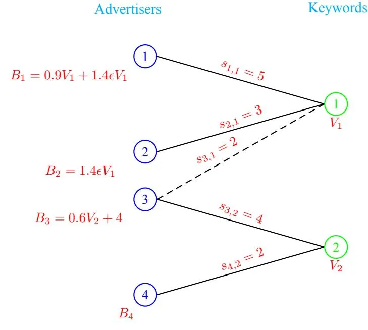
Figure 1: A BMG (without the edge (3,1)) and an extension (with the edge (3,1)), $K=2, \gamma_1=1, \gamma_2=0.7$

5 Advertisers Controlled Broad Match (AdBM)

In this section, we start out with our first goal, that is to provide a reasonable solution concept for the game originating from strategic behavior of advertisers as they try to optimize their budget allocation/splitting across various keywords. We realize that without some reasonable restrictions on the set of available strategies to the advertisers, it is a much harder task to achieve[2]. To this end, we consider a very natural setting for available strategies- (i) first split/allocate the budget across various keywords and then (ii) play the keyword query specific bidding/auction game as long as you have budget left over for that keyword when that query arrives -thereby dividing the overall game in to two stages.

The second stage is exactly the query specific keyword auction and for that stage we can utilize the equilibrium behavior proposed in literature. Therefore, in the second stage, we are restricting the behavior of advertisers in that, given the availability of budget to participate in the auction of a particular query, an advertiser acts rationally but being ignorant about and disregarding the fact that her bidding behavior might effect

her decision in the splitting/allocation of her budget across various keywords in the first stage. For example, in the second stage, for the auction mechanisms currently used by Google and Yahoo! i.e. Generalized Second Price (GSP) Mechanism, we can adopt the solution concept of Symmetric Nash Equilibrium(SNE) proposed in [5, 22]. That is, once the budget is split, for each query all advertisers, with available budgets for the corresponding keyword, bid according to a minimum SNE bid profile. Note that, even for the same keyword, different queries may have different SNE bid profiles because the set of advertisers with available budgets may be different when those queries arrive.

Now, for the first stage i.e. budget splitting, we do not put any restriction on how the advertisers split their budget across various keywords. Each advertiser, knowing the fact that all advertisers will behave according to SNE for keyword queries, chooses her budget splitting so as to maximize her total payoff across all queries of all keywords for the day. Thus, with the restriction on the bidding behavior in second stage, we are left only to analyze the game of splitting the budget across various keywords.

In the spirit of [5, 22] wherein the query specific keyword auction is modeled as a static one shot game of complete information despite its repeated nature in practice, we model the budget splitting too as a static one shot game of complete information because if the budget splitting and bidding process ever stabilize, advertisers will be playing static best responses to their competitors’ strategies. Let us refer to this game as Broad-Match Game. In the following, we search for a reasonable notion of stable budget splitting i.e. a reasonable solution concept for the Broad-Match Game.

5.1 Advertisers’ Best Response Problem and Search for an Appropriate Solution Concept for Broad-Match Game

Let the budget of advertiser i decided for the keyword j be $B_{i,j}$ , then this budget allows her to participate for the first $V_{i,j}$ number of queries for some $V_{i,j} \leq V_j$ . And given a number of queries $V_{i,j}$ for j, there will be a budget requirement from i, depending on the bidding interests of the other bidders, their valuations etc, to participate in the first $V_{i,j}$ queries of j. Thus, there is a one-to-one correspondence between the budget spent on a particular keyword by a bidder and the total number of queries of that keyword starting the first one, that the bidder participates in. Clearly, then the splitting of budget across various keywords can be equivalently considered as deciding on how many queries to participate in, starting their first queries, for those keywords.

Now, with the one shot complete information game modeling, the most natural solution concept to consider is pure Nash equilibrium which in our scenario (i.e. for the Broad-Match Game corresponding to the instance (N, M, K, S, B, V) & BMG $(N, M, \mathcal{E})$ ) can be defined as the matrix of query values $\{V_{i,j}, (i,j) \in \mathcal{E}\}$ such that for each i, given that these values are fixed for all $l \in N - \{i\}$ , no other values of $\{V_{i,j}\}$ gives a better total payoff to the bidder i. Equivalently, it is the matrix of values $\{B_{i,j}, (i,j) \in \mathcal{E}\}$ such that for each i, given that the these values are fixed for all $l \in N - \{i\}$ , no other values of $\{B_{i,j}\}$ gives a better total payoff to the bidder i.

The solution concept of pure Nash equilibrium that we have proposed above requires that the players (i.e. the advertisers) are powerful enough to play the game rationally. In particular, they should be able to compute the best responses to their competitors’ strategies. In the present case, for an advertiser i, it boils down to solving an optimization problem of finding the budget-splitting across various keywords with maximum total payoff, given the budget-splitting of other advertisers. That is, given the values $\{B_{n,j}\}$ for all $n \in \mathbb{N} - \{i\}$ and for all $j \in \mathbb{M}$ , to compute $\{B_{i,j}\}$ yielding maximum payoff for the advertiser i. Of course, the details of BMG is known to every player. To justify this solution concept on algorithmic grounds, it should be essential that this optimization problem of advertiser i, henceforth referred to as Advertisers’ Best Response Problem(AdBRP), should be solvable in time polynomial in N, M, K. Note that we are strictly asking the time complexity to be polynomial in N, M, K and not in $V_j$ ‘s and $B_i$ ‘s. This is because $V_j$ ‘s and $B_i$ ‘s could in general be exponentially larger than N, M, K. In fact, in practice this seem to be the

case as volume of queries could be much larger than the number of advertisers and keywords. Therefore, let us first formulate this optimization problem for advertiser i. Let c(m,j,l) be the (expected) cost of advertiser m for the lth query of the keyword j if she participates in the query l and all the previous queries of the keyword j. Similarly, u(m,j,l) is the (expected) payoff of advertiser m for the lth query of the keyword j if she participates in the query l and all the previous queries of the keyword j. Also define the $marginal\ payoff$ or bang-per-buck for advertiser m for the lth query of keyword j as $\pi(m,j,l) = \frac{u(m,j,l)}{c(m,j,l)}$ . To be able to compute her best response, an advertiser must be able to efficiently compute these values first. For each $(i,j) \in \mathcal{E}$ there are $O(V_j)$ such values and at first glance it seems that the advertiser might take a time polynomial in $V_j$ , i.e. not in strongly polynomial time, to compute these values. However, if we observe carefully there is a lot of redundancy in these values as noted in the following lemma. The idea is that the cost and the payoff of an advertiser for a query of a keyword depends only on the set of advertisers participating in that query and the valuations their of. Therefore, as long as this set is the same these quantities will remain the same.

Lemma 1 For each $i \in \mathbb{N}$ , given the BMG $G = (\mathbb{N}, \mathbb{M}, \mathcal{E})$ and the budget splitting of all advertisers in $\mathbb{N} - \{i\}$ (i.e. the $B_{n,j}$ values for all $n \in \mathbb{N}, j \in \mathbb{M}$ ), there exist non-negative integers $\Lambda_j, z_{j,0}, z_{j,1}, z_{j,2}, \ldots, z_{j,\Lambda_j}$ for all $j \in \{j \in \mathbb{M} : (i,j) \in \mathcal{E}\}$ such that $\Lambda_j = O(N)$ and for all $0 \le \lambda \le \Lambda_j - 1$ ,

$c(i,j,l) = C(i,j,\lambda), u(i,j,l) = U(i,j,\lambda), \pi(i,j,l) = \Pi(i,j,\lambda) \quad \forall z_{j,\lambda} < l \le z_{j,\lambda+1},$

where $C(i,j,\lambda):=c(i,j,z_{j,\lambda}+1), U(i,j,\lambda):=u(i,j,z_{j,\lambda}+1), \Pi(i,j,\lambda):=\pi(i,j,z_{j,\lambda}+1).$ Moreover, all these $\Lambda,z,c,u,\pi$ values can be computed together in $O(MN^2K)$ time.

Proof: The proof follows from Algorithm 5.1 described in the following. The idea in the Algorithm 5.1 is that the cost and the payoff of an advertiser for a query of a keyword depends only on the set of advertisers participating in that query and the valuations their of. Therefore, as long as this set is the same these quantities will remain the same. Further, there can be at most N choices of this set. For the very first query, this set consists of all the advertisers with positive budget for that keyword along with the advertiser i (recall that the budget splittings for other advertisers are given). This set changes when advertisers drop out as their budgets get spent and they no longer have enough amount to buy the next query. This change can occur at most N-1 times. The Algorithm 5.1 tracks exactly when the advertisers drop out and compute the $c, u, \pi$ values accordingly.

The Algorithm 5.1 runs in time $O(N^2K)$ . Initialization requires O(N) and the while loop requires O(NK) in each iteration. There are at most O(N) iteration of the while loop because for every two iteration at least one advertiser drops out. There is a NlogN term, subsumed by $N^2$ , that comes from the need to sort the valuation $s_{i,j}$ ‘s before computing the SNE bid profile.

Algorithm 5.1: QUERY PARTITION(G, j, B_{n,j} \forall n \in \mathbb{N} - \{i\})
  A \leftarrow \{n \in \mathcal{N} - \{i\} : B_{n,j} > 0\}
 z_{j,0} \leftarrow 0
 while A \neq \phi
                 (Compute C(n, j, \lambda) \ \forall n \in A \cup \{i\}
                    and U(i, j, \lambda)
                  \Pi(i,j,\lambda) \leftarrow \frac{U(i,j,\lambda)}{C(i,j,\lambda)}
                if C(i, j, \lambda) = 0
                    then \Pi(i,j,\lambda) \leftarrow \infty
                  y \leftarrow \min_{n \in A} \{ \lfloor \frac{B_{n,j}}{C(n,j,\lambda)} \rfloor \}
                  if y > 0
                      \begin{cases} A_1 \leftarrow A - \{n \in A : \frac{B_{n,j}}{C(n,j,\lambda)} = y\} \\ B_{n,j} \leftarrow B_{n,j} - yC(n,j,\lambda) \ \forall n \in A \\ z_{j,\lambda+1} \leftarrow \min\{z_{j,\lambda} + y, V_j\} \\ A \leftarrow A_1 \\ \lambda \leftarrow \lambda + 1 \end{cases}
     do
                                        \begin{array}{c} \text{if } z_{j,\lambda} = V_j \\ \text{then exit} \end{array}
                                        comment: Exiting the while LOOP
                      else
                  A \leftarrow \{n \in A : \lfloor \frac{B_{n,j}}{C(n,j,\lambda)} \rfloor \neq 0\}
 if A = \phi
 \Lambda_j \leftarrow \lambda
 output (\Lambda_j, \{z_{j,\lambda}\}, \{C(i,j,\lambda)\}, \{U(i,j,\lambda)\}, \{\Pi(i,j,\lambda)\})

Now, using the above lemma we are ready to formulate the AdBRP of advertiser i. Let us define,

$\tilde{U}(i,j,l) = (l-z_{j,\lambda-1})U(i,j,\lambda-1) + \sum_{m=1}^{\lambda-1} (z_{j,m} - z_{j,m-1})U(i,j,m-1) \text{ if } z_{j,\lambda-1} < l \le z_{j,\lambda}.$ (4)

$\tilde{C}(i,j,l) = (l-z_{j,\lambda-1})C(i,j,\lambda-1) + \sum_{m=1}^{\lambda-1} (z_{j,m} - z_{j,m-1})C(i,j,m-1) \text{ if } z_{j,\lambda-1} < l \le z_{j,\lambda}.$ (5)

then the AdBRP is the following optimization problem in non-negative integer variables $x_{i,j}$ ‘s.

$Max \qquad \sum_{(i,j)\in\mathcal{E}} \tilde{U}(i,j,x_{i,j})$

$s.t. \qquad \sum_{(i,j)\in\mathcal{E}} \tilde{C}(i,j,x_{i,j}) \leq B_i$

$0 \leq x_{i,j} \leq V_j \quad \forall \ (i,j) \in \mathcal{E}$

$x_{i,j} \in \mathcal{Z} \quad \forall \ (i,j) \in \mathcal{E}$

$(6)$

It is not hard to see that being a variant of Knapsack Problem (decision version of) AdBRP is NP-hard. Its NP hardness follows from simple restrictions that makes it equivalent to 0-1 Knapsack Problem or Integer Knapsack Problem(IKP) respectively. First, let us restrict all relevant quantities such as budget, utilities and costs to be integer values. Now, in AdBRP, choosing $V_j = 1$ for all $j \in \mathcal{M}$ makes it equivalent to the 0-1 Knapsack Problem. Also, in AdBRP, choosing $\Lambda_j = 1$ for all $j \in \mathcal{M}$ (i.e. a single partition for each keyword) makes it equivalent to the Integer Knapsack Problem.

Now being NP-hard, AdBRP is unlikely to have an efficient algorithm and thus the solution concept based on pure Nash equilibrium does not seem to be reasonable and we should consider weaker notions. One such reasonable solution concept could be that based on local Nash equilibrium, where the advertisers are not required to be so sophisticated and can deviate only locally i.e. by small amounts from the their current strategies. We show that an advertiser’s locally best response can be computed via a greedy algorithm in strongly polynomial time. Further, this equilibrium notion is similar to the user equilibrium/Waldrop equilibrium in routing and transportation science literature[17]. Another solution concept that we explore is motivated by the fact that being a variant of IKP and given that IKP can be approximated well, it may be possible to efficiently compute a pretty good approximation of the advertiser’s best response, and therefore an approximate Nash equilibrium may also make sense. In the following sub-sections we investigate these two solution concepts.

5.2 Broad Match Equilibrium(BME)

Based on our discussion in section 5.1, let us first formally define the equilibrium notion based on local Nash equilibrium and let us refer to it as Broad Match Equilibrium(BME).

Definition 2 Given a BMG $G = (N, M, \mathcal{E})$ , a BME for G is defined as the matrix of query values $\{V_{i,j}\}$ and the budget splitting values $\{B_{i,j}\}$ iff they satisfy the following conditions.

E1) For all i, if $(i,j) \in \mathcal{E}$ with $V_{i,j} > 0$ , and $(i,l) \in \mathcal{E}$ which is not query-saturated meaning $V_{i,j} < V_j$ then $MP_{i,j}^- := \frac{u(i,j,V_{i,j})}{c(i,j,V_{i,j})} \ge MP_{i,l}^+ := \frac{u(i,l,V_{i,l}+1)}{c(i,l,V_{i,l}+1)}$ i.e. the advertiser i does not have an incentive to deviate locally from keyword j to keyword l.

E2) For all i*,* i spends her total budget Bⁱ (on some keyword or the other) unless each (i, j) ∈ E is either query-saturated (i.e. Vi,j = V^j ) or budget-saturated meaning that the left over budget of advertiser i for keyword j is insufficient to buy the next query of j*.*

Now given the {Vn,j} and {Bn,j} values for all n ∈ N − {i}, the locally best response problem ( local AdBRP) for i is to compute a set of {Vi,j} and {Bi,j} values such that they satisfy all conditions in the above definition of BME. We show in the following theorem that the local AdBRP can be computed efficiently. Thus, BME is indeed a reasonable solution concept for the Broad-Match Game.

The idea in the proof of Theorem 3 is to first partition the queries across various keywords via Lemma 1 so that the payoff, cost, and marginal payoff of i is the same for all queries in a given partition. Then, in a GREEDY ALLOCATION PHASE, to greedily distribute the budgets across various keywords moving from one partition to another. Finally, in a GREEDY READJUSTMENT PHASE, if there is an edge (i, l) which is not stable (i.e. the advertiser i could profitably deviate locally to this edge from another edge(s)), a reverse greedy approach would take budgets from edge with minimum marginal payoff and put it to (i, l) until (i, l) becomes stable, again via moving from partition to partition. Since we always move from partition to partition and a partition is visited at most once in each of the above two phases, and there are at most O(N) partitions per keyword, this algorithm is efficient.

Theorem 3 There is a strongly polynomial time algorithm for local AdBRP.

Proof: The proof follows from the Algorithm 5.2 provided in the following. The Algorithm 5.2 first partitions the queries across various keywords so that the payoff, cost, and marginal payoff of i is the same for all queries in a given partition. This is computed via Algorithm 5.1 which takes O(MN2K) time. Initialization takes O(M) time. In the GREEDY ALLOCATION PHASE, the algorithm greedily distributes the budgets across various keywords moving from one partition to another. Each iteration of the while loop in this phase takes O(M) time and since there are O(MN) partitions the total time taken for this loop is O(M2N). GREEDY READJUSTMENT PHASE first checks if there is any edge (i, l) which is not stable i.e. the advertiser i could profitably deviate locally to this edge from another edge(s). It is not hard to see that at the end of GREEDY ALLOCATION PHASE, there can be at most one such edge (ref. Lemma 4). If there is such an edge, this phase adjusts the budget to make this edge stable without making any other edge unstable. This is achieved via a reverse greedy approach taking budgets from edge with minimum marginal payoff and putting to (i, l) until (i, l) becomes stable, again via moving from partition to partition. Thus, Algorithm 5.2 correctly computes a locally best response for advertiser i*.* The while loop in this readjustment phase also terminates in O(MN) iterations and therefore this phase takes total of O(M2N) time. Hence, the running time of Algorithm 5.2 is $O(MN^2K + M^2N)$ i.e. strongly polynomial time.

Algorithm 5.2: Greedy Budget Splitting $(G, B_{n,j} \forall n \in \mathbb{N} - \{i\}, j \in \mathbb{M})$

$J_i = \{ j \in \mathcal{M} : (i, j) \in \mathcal{E} \}$

comment: Computing $\Lambda, z, C, U, \Pi$ values for all relevant j’s

for each $j \in J_i$

do Query Partition $(G, j, B_{n,j} \forall n \in \mathbb{N} - \{i\})$

comment: Initialization

$\begin{aligned} & \lambda_j \leftarrow 0 \ \, \forall j \in J_i \\ & y_j \leftarrow z_{j,1} \ \, \forall j \in J_i \\ & C_{i,j} \leftarrow 0, B_{i,j} \leftarrow 0, V_{i,j} \leftarrow 0 \ \, \forall j \in J_i \\ & C_i \leftarrow 0 \end{aligned}$

comment: GREEDY ALLOCATION PHASE

while $J_i \neq \phi$

$L \leftarrow arg \max_{i \in J_i} \Pi(i, j, \lambda_i)$ if there are more than one such index take the minimum one

\begin{aligned} & \textbf{if } C_i + y_L C(i, L, \lambda_L) > B_i \\ & \begin{cases} y \leftarrow \lfloor \frac{B_i - C_i}{C(i, L, \lambda_L)} \rfloor \\ V_{i,L} \leftarrow V_{i,L} + y \\ B_{i,L} \leftarrow B_{i,L} + (B_i - C_i) \\ C_{i,L} \leftarrow C_{i,L} + yC(i, L, \lambda_L) \\ C_i \leftarrow C_i + yC(i, L, \lambda_L) \end{aligned} \end{aligned}

exit comment: Exiting the while LOOP $\begin{cases} B_{i,L} \leftarrow B_{i,L} + y_L C(i,L,\lambda_L) \\ C_{i,L} \leftarrow C_{i,L} + y_L C(i,L,\lambda_L) \\ C_{i,L} \leftarrow C_{i,L} + y_L C(i,L,\lambda_L) \\ C_i \leftarrow C_i + y_L C(i,L,\lambda_L) \end{cases}$ else $\begin{cases} \mathbf{if} \ \lambda_L = \Lambda_j - 1 \\ \mathbf{comment:} \ \text{ i.e. no more queries for } L \text{ is left} \end{cases}$ then $\begin{cases} J_i \leftarrow J_i - \{L\} \\ \lambda_L \leftarrow \lambda_L + 1 \\ \mathbf{else} \end{cases}$

$\begin{cases} y_L \leftarrow z_{L,\lambda_L+1} - z_{L,\lambda_L} \\ \lambda_L \leftarrow \lambda_L + 1 \end{cases}$

\begin{split} &\textbf{then } \begin{cases} J_i \leftarrow J_i - \{L\} \\ \lambda_L \leftarrow \lambda_L + 1 \end{cases} \\ &\textbf{else } \begin{cases} y_L \leftarrow z_{L,\lambda_L+1} - z_{L,\lambda_L} \\ \lambda_L \leftarrow \lambda_L + 1 \end{cases}

comment: GREEDY READJUSTMENT PHASE

$J_i \leftarrow \{j : (i,j) \in \mathcal{E} \text{ and } V_{i,j} > 0\}$

$l \leftarrow \{l \in \mathcal{M} : (i, l) \in \mathcal{E} \text{ and } \exists j \in J_i - \{l\} \text{ s.t. } MP_{i,l}^+ > MP_{i,j}^- \}$

comment: there can be at most one such l (ref. Lemma 4)

if such an l does not exist then return $(\{V_{i,j}\}, \{B_{i,j}\})$ comment: Readjustment not required

output $(\{V_{i,j}\}, \{B_{i,j}\})$

while $\lambda_l < \Lambda_l$ and $MP_{i,l}^+ > \min_{j \in J_i - \{l\}} MP_{i,j}^-$

\begin{aligned} & \text{while } \lambda_{l} < \Lambda_{l} \text{ and } MP_{i,l}^{+} > \min_{j \in J_{i} - \{l\}} MP_{i,j}^{-} \\ & j \leftarrow \arg \min_{j \in J_{i} - \{l\}} MP_{i,j}^{-} \\ & y \leftarrow \left\lfloor \frac{(V_{i,j} - z_{j,\lambda_{j} - 1})C(i,j,\lambda_{j} - 1) + (B_{i,j} - C_{i,j}) + (B_{i,l} - C_{i,l})}{C(i,l,\lambda_{l})} \right\rfloor \\ & \text{if } y < z_{l,\lambda_{l} + 1} - V_{i,l} \\ & \begin{bmatrix} B_{i,l} \leftarrow B_{i,l} + (V_{i,j} - z_{j,\lambda_{j} - 1})C(i,j,\lambda_{j} - 1) \\ + (B_{i,j} - C_{i,j}) \\ C_{i,j} \leftarrow C_{i,j} - (V_{i,j} - z_{j,\lambda_{j} - 1})C(i,j,\lambda_{j} - 1) \\ B_{i,j} \leftarrow C_{i,j} + yC(i,l,\lambda_{l}) \\ \lambda_{j} \leftarrow \lambda_{j} - 1 \\ V_{i,j} \leftarrow z_{j,\lambda_{j}} \\ & \text{if } V_{i,j} = 0 \\ \text{then } J_{i} \leftarrow J_{i} - \{j\} \\ & V_{i,l} \leftarrow V_{i,l} + y \end{aligned}

$\begin{cases} \tilde{y} \leftarrow \left\lceil \frac{(z_{l,\lambda_{l} + 1} - V_{i,l})C(i,l,\lambda_{l}) - (B_{i,j} - C_{i,j}) - (B_{i,l} - C_{i,l})}{C(i,j,\lambda_{j} - 1)} \right\rceil \\ C_{i,j} \leftarrow C_{i,j} - \tilde{y}C(i,j,\lambda_{j} - 1) \\ B_{i,j} \leftarrow B_{i,j} + \left[ (z_{l,\lambda_{l} + 1} - V_{i,l})C(i,l,\lambda_{l}) - (B_{i,l} - C_{i,l}) \right] \\ C_{i,l} \leftarrow C_{i,l} + (z_{l,\lambda_{l} + 1} - V_{i,l})C(i,l,\lambda_{l}) \\ B_{i,l} \leftarrow C_{i,l} \end{cases}$

\begin{cases} \tilde{y} = V_{i,j} - \tilde{y}_{j,\lambda_{j} - 1} \\ V_{i,j} \leftarrow \tilde{z}_{j,\lambda_{j}} \\ \text{if } \tilde{y} = V_{i,j} - z_{j,\lambda_{j} - 1} \\ V_{i,j} \leftarrow \tilde{z}_{j,\lambda_{j}} \\ \text{if } V_{i,j} \leftarrow \tilde{z}_{j,\lambda_{j}} \end{cases} \end{cases}

$\begin{cases} \lambda_{l} \leftarrow \lambda_{l} + 1 \\ V_{i,l} \leftarrow z_{l,\lambda_{l}} \end{cases}$

\begin{cases} \lambda_{l} \leftarrow \lambda_{l} + 1 \\ V_{i,l} \leftarrow z_{l,\lambda_{l}} \end{cases} \end{cases}

Lemma 4 At the end of GREEDY ALLOCATION PHASE of Algorithm 5.2, there can be at most one unstable edge, that is

$|\left\{l \in \mathcal{M}: (i,l) \in \mathcal{E} \ \textit{and} \ \exists j \ s.t. (i,j) \in \mathcal{E}, V_{i,j} > 0 \ \& \ MP_{i,l}^{+} > MP_{i,j}^{-}\right\}| < 1.$

Proof: We will provide a proof by contradiction. If possible, let there be two unstable edges namely (i,l) and (i,m), thus there exist an edge $(i,j) \in \mathcal{E}$ with $V_{i,j} > 0$ such that $MP_{i,l}^+ > MP_{i,j}^-$ and $MP_{i,m}^+ > MP_{i,j}^-$ . Note that there could be many such choices of j, let us choose the one with the minimum value of $MP_{i,j}^-$ . Thus, in the Figure 2, we are given that $\pi_1 < \min\{\pi_3, \pi_5\}$ . Since the greedy allocation phase fills up ( or selects) the partitions with higher values first, starting the markers on the first partition of all the keywords, there must be partitions with values $\pi_2 \le \pi_1$ and $\pi_4 \le \pi_1$ as shown in Figure 2, otherwise all partitions of (i,l) before and with the value $\pi_3$ must have been filled/selected before the partition with value $\pi_1$ and similarly for all partitions of (i,m) before and with the value $\pi_5$ . WLog let the partition with the value $\pi_2$ is filled before that with $\pi_4$ . Therefore, $\pi_3 \le \pi_4$ otherwise the open partition ( i.e. the one not yet completely filled ) with value $\pi_3$ would have been filled before $\pi_4$ . Further, by using $\pi_2 \le \pi_1$ and $\pi_1 < \pi_3$ we get $\pi_2 < \pi_3$ and consequently $\pi_2 < \pi_4$ . As before we can again argue that there exist a partition with value $\pi_6 < \pi_2$ but we must also have $\pi_3 \le \pi_6$ otherwise the open partition with value $\pi_3$ would have been filled before $\pi_6$ . But this implies $\pi_3 < \pi_2$ which is a contradiction.

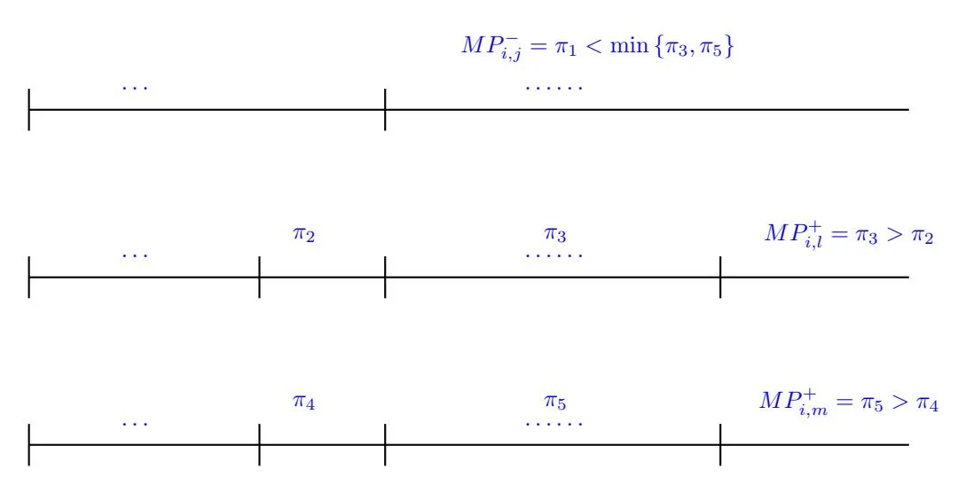
Figure 2: There can not be two unstable edges at the end of GREEDY ALLOCATION PHASE in Algorithm 5.2. The $\pi$ values shown in the figure are the marginal payoffs of i in the respective partitions. ”…” shown between two partitions indicate that there could be several or no partitions between these partitions.

One might also like to consider another natural strongly polynomial time greedy algorithm based on the algorithm for fractional knapsack problem, considering each keyword as an item, total payoff (from all the queries that can be bought within the budget constraint) as the value and the corresponding total cost as the size, sorting the keywords by effective marginal payoffs i.e. $\frac{\text{total payoff}}{\text{total cost}}$ , and greedily selecting the keywords until budget is exhausted. However, it can be shown (Figure 4) that this greedy approach does not always lead to a locally best response of an advertiser i.e. there are examples where the solution given by this algorithm is not stable and the advertiser can improve her payoff by local deviation. Further, it is not clear whether some readjustment procedure as in the GREEDY READJUSTMENT PHASE of the Algorithm

5.2 could be applied to make such solutions stable. In this paper, we have not explored this direction in details and it might be interesting to make this algorithm work, if possible, by some suitable readjustment, and compare its performance with to that of Algorithm 5.2. For an initial insight, first note that, in the example given in Figure 3, the marginal payoffs for a keyword are increasing with the partition number i.e. $\Pi(i,2,1)>\Pi(i,2,0)$ . The effective marginal payoff for keyword 2 is $\frac{4.5V_1-7.5}{2V_1-2}>2$ when $V_1>7$ and this algorithms therefore spends all budget on keyword 2, giving a payoff better than Algorithm 5.2. Also, it is a stable solution because $MP_{i,2}^-=3>2=MP_{i,1}^+$ . In fact, in this particular example it is the global optimum. In general, clearly when this algorithm returns a stable solution without a need for readjustment, it always chooses a better budget splitting than Algorithm 5.2, however as we give an example below in the Figure 4, it might not always return a stable solution.

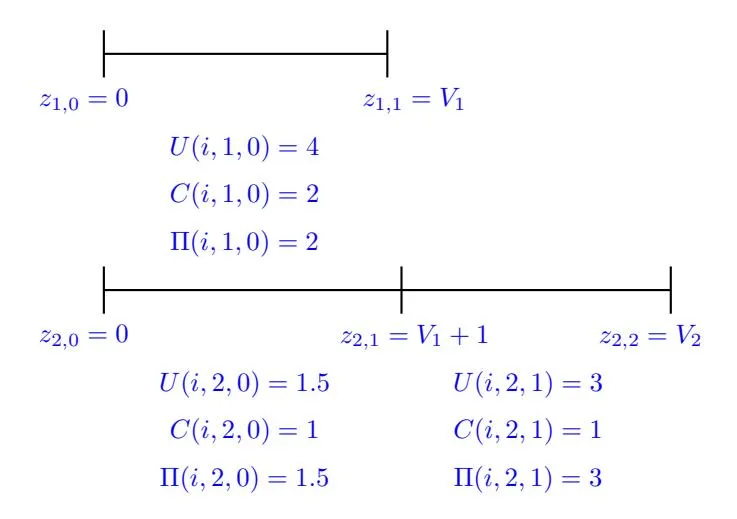
Figure 3: Let $B_i = 2(V_1 - 1)$ and $V_2 \ge 2V_1 - 2$ . Algorithm 5.2 outputs $(B_{i,1} = B_i, B_{i,2} = 0, V_{i,1} = V_1 - 1, V_{i,2} = 0)$ with total payoff of $4V_1 - 4$ to the advertiser. However, the splitting $(B_{i,1} = 0, B_{i,2} = B_i, V_{i,1} = 0, V_{i,2} = 2V_1 - 2)$ gives a total payoff of $4.5V_1 - 7.5 > 4V_1 - 4$ when $V_1 > 7$ .

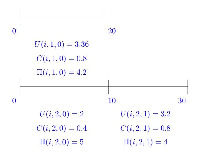
Figure 4: Greedy fractional knapsack algorithm may not return a stable solution. $B_i=12$ . This algorithm allocates all the budget to the keyword 2 as the effective marginal payoffs is $\frac{2\times 10+3.2\times 10}{0.4\times 10+0.8\times 10}=\frac{52}{12}$ which is greater than that of keyword 1 which is $\frac{3.36\times 15}{0.8\times 15}=\frac{50.4}{12}$ . However, the edge (i,1) is now unstable as $MP_{i,1}^+=4.2>4=MP_{i,2}^-$ .

5.3 Approximate Nash Equilibrium( $\epsilon$ -NE)

Let us first define the approximate Nash equilibrium for our setting as follows.

Definition 5 Given a BMG $G = (\mathcal{N}, \mathcal{M}, \mathcal{E})$ , an $\epsilon$ -NE for G is defined as the matrix of query values $\{V_{i,j}\}$ and the budget splitting values $\{B_{i,j}\}$ such that for all $i, \sum_{(i,j)\in\mathcal{E}} \tilde{U}(i,j,V_{i,j}) \geq (1-\epsilon) \sum_{(i,j)\in\mathcal{E}} \tilde{U}(i,j,\tilde{V}_{i,j})$ for all alternative strategy choices $\{\tilde{V}_{i,j}\}$ of advertiser i that satisfies the constraints in Equation 6.

Now given the $\{V_{n,j}\}$ and $\{B_{n,j}\}$ values for all $n \in \mathbb{N} - \{i\}$ , the approximate best response problem ( $\epsilon$ -AdBRP) for i is to compute a set of $\{V_{i,j}\}$ and $\{B_{i,j}\}$ values satisfying the conditions in the above definition of $\epsilon$ -NE.

As we mentioned earlier, the AdBRP is a variant of knapsack problem and we also know that the later can be approximated very well. Further, if we expect to get an FPTAS for AdBRP, we would expect that it also admits a pseudo-polynomial time algorithm (i.e. polynomial in N, M, K, $V_j$ ‘s, and $B_i$ ‘s) as well [23, 16]. Furthermore, all known pseudo-polynomial time algorithms for NP-hard problems are based on dynamic programming [23, 16]. Therefore, naturally we try a similar approach. Perhaps not surprisingly, we design a pseudo-polynomial time algorithm for AdBRP. However, unlike the case of standard knapsack problems[8, 10, 23, 16], this algorithm does not immediately give a FPTAS due to difficulty in handling the volume of queries and because for a given keyword (i.e. the item) queries may have different costs and utilities (i.e. all units of an item are not equivalent in cost and value) etc. Nevertheless, by judiciously utilizing the properties of the optimum and a double-layered approximation we will indeed present a FPTAS for AdBRP (Theorem 6). We will devote the Sections 5.3.1, 5.3.2, 5.3.3 on developing a FPTAS for AdBRP.

Theorem 6 There is a FPTAS for AdBRP.

Thus, $\epsilon$ -NE is indeed another reasonable solution concept for the Broad-Match Game.

5.3.1 A Pseudo Polynomial Time Algorithm for AdBRP

Without loss of generality, first let us assume that all relevant parameters such as budget, utilities, and costs are integer valued. This can be achieved by suitable approximation to rational numbers and then by appropriate multiplication factors, without significant increase in instance size.

Let P be the maximum total utility that the advertiser i can derive from a single keyword i.e. from any one of the $j \in \mathcal{M}$ while respecting her budget constraint. Therefore, MP is a trivial upperbound on the total utility that can be achieved by any solution (i.e. any choice of feasible $x_{i,l}$ ‘s). For $j \in \mathcal{M}$ and $p = 1, 2, \ldots, MP$ let us define,

$A(j,p) = \begin{cases} &\textit{Min } \sum_{l=1}^{j} \tilde{C}(i,l,x_{i,l}) \\ &\textit{s.t. } \sum_{l=1}^{j} \tilde{U}(i,l,x_{i,l}) \geq p \\ &0 \leq x_{i,l} \leq V_l \quad \text{for } l=1,2,\ldots,j \\ &x_{i,l} \in \mathcal{Z} \quad \text{for } l=1,2,\ldots,j \end{cases}$

$\infty \quad \text{if no solution to the above minimization problem exists}$

$(7)$

Clearly, the values A(1,p) for all $p=1,2,\ldots,MP$ can each be efficiently computed (in $O(Nlog(V_1))$ time) by utilizing the partition structure as per Lemma 1 and the Equations 4 and 5. The term $log(V_1)$

instead of $V_1$ comes from the the fact that it is enough to perform a binary search inside a partition for an appropriate $x_{i,1}$ . Therefore, the values A(1,p) for all $p=1,2,\ldots,MP$ can be together computed in $O(Nlog(V_1)MP)$ time. Let $V=\sum_{j\in\mathcal{M}}V_j$ . Now, A(j,p) for all $j=2,3,\ldots,M$ and $p=1,2,\ldots,MP$ can be computed together in $O(M^2PNV)$ using following recurrence relation. Further, for each choice of $j=1,2,3,\ldots,M$ and $p=1,2,\ldots,MP$ , we also compute and store the set of $x_{i,j}$ ‘s values that achieves the value of A(j,p), and this task can be performed in same order of time complexity.

$A(j+1,p) \ = \begin{cases} &\textit{Min} \ \sum_{l=1}^{j} \tilde{C}(i,l,x_{i,l}) + \tilde{C}(i,j+1,x_{i,j+1}) \\ &\textit{s.t.} \ \sum_{l=1}^{j} \tilde{U}(i,l,x_{i,l}) + \tilde{U}(i,j+1,x_{i,j+1}) \geq p \\ &0 \leq x_{i,l} \leq V_{l} \ \text{ for } l=1,2,\ldots,j+1 \\ &x_{i,l} \in \mathcal{Z} \ \text{ for } l=1,2,\ldots,j+1 \end{cases}$

$= \min_{x_{i,j+1} \in \{0,1,2,\dots,V_{j+1}\}: \tilde{U}(i,j+1,x_{i,j+1}) \leq p} \left\{ \tilde{C}(i,j+1,x_{i,j+1}) + A(j,p-\tilde{U}(i,j+1,x_{i,j+1})) \right\}$

After computing the A(j, p)‘s, we can obtain the solution of AdBRP and the optimum value via

$OPT = \max_{p=1,2,...,MP} \{ p : A(M,p) \le B_i \}.$ (9)

Thus, we have a pseudo-polynomial time algorithm for AdBRP.

5.3.2 A Pseudo Polynomial Time Approximation Scheme for AdBRP

Now, we will convert the pseudo polytime algorithm of Section 5.3.1 to an approximation scheme by appropriately rounding the payoffs of the advertisers. Let us call this scheme AS1.

For a given $\epsilon>0$ , let $T=\frac{\epsilon P}{M}$ and let us round the utility functions from $\tilde{U}(i,l,x_{i,l})$ to $\tilde{U}'(i,l,x_{i,l})=\lfloor\frac{\tilde{U}(i,l,x_{i,l})}{T}\rfloor$ . Now, let us use the above dynamic programming algorithm by replacing the upper bound on utility P to $\lfloor\frac{P}{T}\rfloor$ and utilities $\tilde{U}(i,l,x_{i,l})$ to $\tilde{U}'(i,l,x_{i,l})$ . Let us denote the solution returned as $V'_{i,j}$ i.e. the optimum of the problem after above rounding is attained at $x_{i,j}=V'_{i,j}, j\in \mathcal{M}$ . Correspondingly, let the optimal solution without any rounding is $V_{i,j}, j\in \mathcal{M}$ . Note that the values $\{V_{i,j}\}$ are still feasible for the rounded problem.

Now since $\{V'_{i,j}\}$ is optimal for the rounded problem we have

$\sum_{j \in \mathcal{M}} \tilde{U}'(i, j, V'_{i,j}) \geq \sum_{j \in \mathcal{M}} \tilde{U}'(i, j, V_{i,j})$

$\geq \sum_{j \in \mathcal{M}} \left(\frac{\tilde{U}(i, j, V_{i,j})}{T} - 1\right)$

$= \sum_{j \in \mathcal{M}} \frac{\tilde{U}(i, j, V_{i,j})}{T} - M$ (10)

Further, using the inequality 10, we can get

$\sum_{j \in \mathcal{M}} \tilde{U}(i, j, V'_{i,j}) \geq \sum_{j \in \mathcal{M}} T\tilde{U}'(i, j, V'_{i,j})$

$\geq \sum_{j \in \mathcal{M}} \tilde{U}(i, j, V_{i,j}) - TM$

$= \sum_{j \in \mathcal{M}} \tilde{U}(i, j, V_{i,j}) - \epsilon P$

$\geq (1 - \epsilon) \sum_{j \in \mathcal{M}} \tilde{U}(i, j, V_{i,j})$

where the last inequality is implied by the fact that the optimal value without rounding will at least be the maximum derived from a single keyword i.e. $\sum_{j\in\mathcal{M}} \tilde{U}(i,j,V_{i,j}) \geq P$ . Therefore, the $\{V'_{i,j}\}$ gives an $(1-\epsilon)$ approximation to the advertiser i’s best response. The time complexity of the dynamic programming applied to obtain the solution $\{V'_{i,j}\}$ is $O(M^2\lfloor \frac{P}{T} \rfloor NV) = O(M^2N(\lfloor \frac{M}{\epsilon} \rfloor)V)$ which is polynomial in N, M, V and $\frac{1}{\epsilon}$ . Note that this scheme is still pseudo polynomial due to appearance of V. This terms appears because when we build up the dynamic programming table we need to use the Equation 8. Nevertheless, this algorithm will be helpful in designing our FPTAS.

5.3.3 FPTAS for AdBRP

Now using the approximation scheme AS1 and by judiciously truncating set of possible query values we will present an FPTAS for AdBRP. Let us first note that for each keyword only the number of queries, starting the first one, that can be bought under budget constraint $B_i$ are feasible. Therefore, for the ease of notation, without loss of generality, we can assume that $V_j$ is infact the maximum number of queries that can be bought under budget constraint meaning all possible queries of a particular keyword are feasible if i wanted to spend her total budget on this keyword. Let $V = \sum_{j \in M} V_j$ . Also, without loss of generality we have $U(i, j, \lambda) > 0$ for all $\lambda$ and j such that $(i, j) \in \mathcal{E}$ .

Now, we perform a first layer of approximation by judiciously truncating the set of possible query values to obtain Lemma 8. Lemma 7 is just a warmup.

Lemma 7 There is a feasible solution $\{\hat{V}_{i,j}\}$ of AdBRP with the total utility $\hat{OPT}$ satisfying the following properties where OPT is the total utility for the optimal solution of AdBRP:

• At most for one $j \in M$ , $\hat{V}_{i,j} \notin \{z_{j,0}, z_{j,1}, z_{j,2}, \dots, z_{j,\Lambda_j}\}$
• $\hat{OPT} \geq (1 \delta)OPT$ where $\delta = \max_{j,\lambda} \frac{U(i,j,\lambda)}{OPT}$

Proof:

Consider all the keywords j for which $V_{i,j} \notin \{z_{j,0}, z_{j,1}, z_{j,2}, \ldots, z_{j,\Lambda_j}\}$ . Now among these keywords, for the keywords with the maximum value of $\pi(i,j,V_{i,j})$ , move the budget from one to the other unless all keywords of such type except one satisfies the above condition, this moving around of budgets among the keywords with the same value of $\pi(i,j,V_{i,j})$ does not change the total utility. Thus, we can safely assume that there is a single keyword satisfying $V_{i,j} \notin \{z_{j,0}, z_{j,1}, z_{j,2}, \ldots, z_{j,\Lambda_j}\}$ with the maximum value of $\pi(i,j,V_{i,j})$ and say its l. Further, we can move budget from all other keywords satisfying $V_{i,j} \notin \{z_{j,0}, z_{j,1}, z_{j,2}, \ldots, z_{j,\Lambda_j}\}$ , while losing at

most $u(i, l, V_{i,l})$ . This is because while doing this reallocation we lose only when we do not have enough budget to move to buy the next query of l.

Lemma 8 For every given parameter $\epsilon < 1$ , there is a feasible solution $\{\hat{V}_{i,j}\}$ of AdBRP with the total utility $\hat{OPT}$ satisfying the following properties where OPT is the total utility for the optimal solution of AdBRP:

• $\hat{OPT} > (1 \epsilon^2)OPT$
• $\hat{V}_{i,j} \in \{y_{j,0}, y_{j,1}, y_{j,2}, \dots, y_{j,n_j}\}$ for all $j \in M$ where the $y_{j,.}$ values are defined as follows:

for each partition $\lambda=1,2,\ldots,\Lambda_j$ of the keyword j let $z_{j,\lambda}-z_{j,\lambda-1}=a\lceil\frac{M}{\epsilon^2}\rceil+b$ where a and b are non-negative integers and $b<\lceil\frac{M}{\epsilon^2}\rceil$ (recall that $z_{j,\lambda}-z_{j,\lambda-1}$ is the size of partition $\lambda$ ). Now divide the partition $\lambda$ in to $\min\{a,1\}$ . $\lceil\frac{M}{\epsilon^2}\rceil+b$ sub-partitions, the first $\min\{a,1\}$ . $\lceil\frac{M}{\epsilon^2}\rceil$ sub-partitions being of size a queries each and the next b partitions each of size 1 query each. Define $y_{j,0}=0$ and $y_{j,1},y_{j,2},\ldots,y_{j,n_j}$ as the end points of the sub-partitions created as above.

Proof: Clearly, each partition is divided in to at most $2\lceil \frac{M}{\epsilon^2} \rceil$ sub-partitions and since $\Lambda_j = O(N)$ we obtain $n_j = O(\frac{NM}{\epsilon^2})$ .

Let $\{V_{i,j}\}$ be an optimal solution for AdBRP, then we find a solution $\{\hat{V}_{i,j}\}$ as follows:

• if $V_{i,j} \in \{y_{j,0}, y_{j,1}, y_{j,2}, \dots, y_{j,n_j}\}$ then $\hat{V}_{i,j} = V_{i,j}$ , therefore we do not lose anything in total utility coming from keyword j by moving from $V_{i,j}$ to $\hat{V}_{i,j}$ .
• if $V_{i,j} \notin \{y_{j,0}, y_{j,1}, y_{j,2}, \dots, y_{j,n_j}\}$ then define $\hat{V}_{i,j}$ to be the maximum value among $\{y_{j,0}, y_{j,1}, y_{j,2}, \dots, y_{j,n_j}\}$ which is smaller than $V_{i,j}$ . Note that this case arises only when $V_{i,j}$ comes from a sub-partition of size a>1 and in that case there are at least $\lceil \frac{M}{\epsilon^2} \rceil$ sub-partitions of size a with the same utility value $u(i,j,V_{i,j})$ for each query in those sub-partitions. The maximum utility that we can lose by truncating $V_{i,j}$ to $\hat{V}_{i,j}$ is $\leq a\ u(i,j,V_{i,j}) \leq \frac{1}{\lceil \frac{M}{\epsilon^2} \rceil} \left( \lceil \frac{M}{\epsilon^2} \rceil \ a\ u(i,j,V_{i,j}) \right) \leq \frac{1}{\lceil \frac{M}{\epsilon^2} \rceil} OPT \leq \frac{\epsilon^2}{M} OPT$ .

Note that the way we have constructed $\{\hat{V}_{i,j}\}$ , it satisfies the budget constraint of the advertiser i because $\hat{V}_{i,j} \leq V_{i,j}$ and hence $\{\hat{V}_{i,j}\}$ is a feasible solution of AdBRP. Now, across all the keywords we can lose at most M $\frac{\epsilon^2}{M}OPT$ i.e. $\epsilon^2OPT$ by truncating the optimal solution $\{V_{i,j}\}$ to the feasible solution $\{\hat{V}_{i,j}\}$ .

Now we perform a second layer of approximation by applying AS1 with truncated set of possible query values as per Lemma 8. We present this approximation algorithm called AS2 in the following.

• 1. Divide each partition of each keyword in to several sub-partitions as follows (same as in the proof of Lemma 8). For each partition $\lambda=1,2,\ldots,\Lambda_j$ of the keyword j let $z_{j,\lambda}-z_{j,\lambda-1}=a\lceil\frac{M}{\epsilon^2}\rceil+b$ where a and b are non-negative integers and $b<\lceil\frac{M}{\epsilon^2}\rceil$ (recall that $z_{j,\lambda}-z_{j,\lambda-1}$ is the size of partition $\lambda$ ). Now divide the partition $\lambda$ in to $min\{a,1\}.\lceil\frac{M}{\epsilon^2}\rceil+b$ sub-partitions, the first $min\{a,1\}.\lceil\frac{M}{\epsilon^2}\rceil$ sub-partitions being of size a queries each and the next b partitions each of size 1 query each. Define $y_{j,0}=0$ and $y_{j,1},y_{j,2},\ldots,y_{j,n_j}$ as the end points of the sub-partitions created as above.
• 2. Apply ASI by restricting the query values to take values only from the set $\{y_{j,0}, y_{j,1}, y_{j,2}, \dots, y_{j,n_j}\}$ i.e. by changing the recurrence relation 8 to

$A(j+1,p) = \min_{x_{i,j+1} \in \{y_{j,0}, y_{j,1}, y_{j,2}, \dots, y_{j,n_j}\}: \tilde{U}(i,j+1,x_{i,j+1}) \le p} \left\{ \tilde{C}(i,j+1,x_{i,j+1}) + A(j,p-\tilde{U}(i,j+1,x_{i,j+1})) \right\}$

$(11)$

and with the error parameter $\tilde{\epsilon}$ , where $\frac{1}{\tilde{\epsilon}}=\frac{1}{\epsilon}+1\leq\frac{2}{\epsilon}.$

The total utility of the solution returned by the algorithm AS2 is

$\geq (1 - \tilde{\epsilon})(1 - \epsilon^2)OPT = (1 - \frac{\epsilon}{1 + \epsilon})(1 - \epsilon^2)OPT = (1 - \epsilon)OPT.$

The time complexity in constructing the sub-partitions is $O(\frac{NM}{\epsilon^2})$ and that of applying ASI on the truncated set of query values $\{y_{j,0},y_{j,1},y_{j,2},\ldots,y_{j,n_j}\}$ is $O(M^2N(\lfloor\frac{M}{\epsilon}\rfloor)\frac{NM}{\epsilon^2})=O(\frac{M^4N^2}{\epsilon^3})$ as $\frac{1}{\epsilon}=\frac{1}{\epsilon}+1\leq \frac{2}{\epsilon}=O(\frac{1}{\epsilon})$ . Therefore, AS2 is indeed a FPTAS for AdBRP.

5.4 To Broad-match or not to Broad-match

In this section, we start out with a very important observation in the following theorem.

Theorem 9 A BMG does not necessarily have a unique BME and the different BMEs can yield different revenues to the auctioneer. Moreover, in one of them the auctioneer loses while in the other one it gains in terms of revenue.

The Theorem 9 leaves the auctioneer in a dilemma about whether he should broad-match or not. If he could somehow predict which choice of broad match lead to a revenue improvement for him and which not, he could potentially choose the ones leading to a revenue improvement. This brings forth one of the big questions left open in this paper, that is of efficiently computing a $BME / \epsilon - NE$ , if one exists, given a choice of broad match. We plan to explore it in our future works. The proof of the above theorem follows from examples constructed in Figures 5, 6, 7. Further, in all the examples we take K = 2, $\gamma_1 = 1$ , $\gamma_2 = 0.7$ .

We also note several other observations such as

• introducing an edge may or may not shift the BME ( See Figures 8,9)
• introducing an edge can shift the BME to one yielding less revenue to the auctioneer, as well as, to one with less efficiency i.e. social welfare (See Figure 1, 9)
• introducing new edges can shift the BME to one yielding more revenue to the auctioneer (See Figures 9, 5, 6, 7)
• unlike in Figure 9, an extension of a BMG may not have a BME where for all nodes the degree is the same as in the BME for the base BMG. See Figures 1, 6, 7.

It is instructive to note that all the above observations (including Theorem 9) continue to hold under the solution concept of $\epsilon$ -NE.

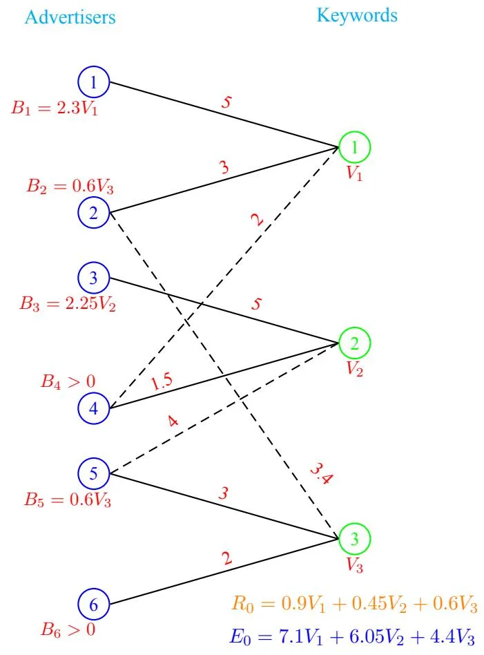
Figure 5: A BMG (without dashed edges) and its extension (with dashed edges). The values shown along the edges are si,j respectively. Further, note that it is a good broad-match as valuations si,j of an advertiser along new edges is greater than her valuation along old edges.

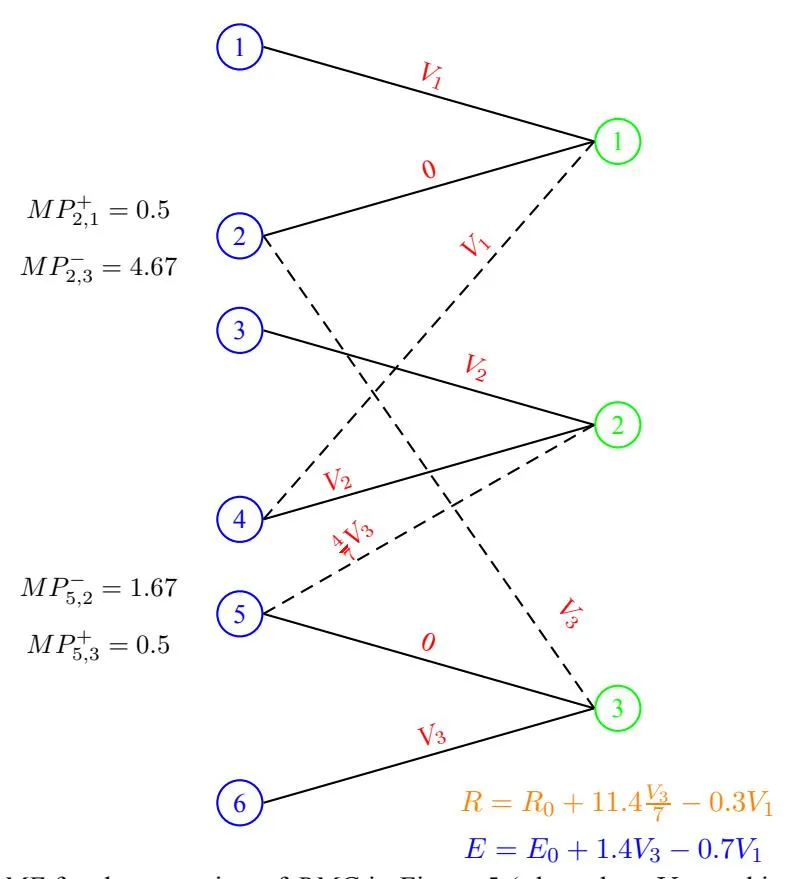
Figure 6: One BME for the extension of BMG in Figure 5 ( the values $V_{i,j}$ at this BME are shown along corresponding edges).

Not a pure Nash equilibrium but an $\epsilon\text{-NE}$ for $\epsilon \geq 0.15.$

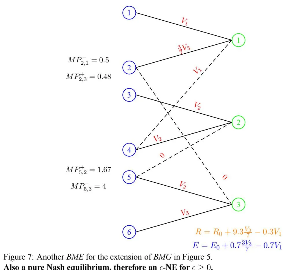
Also a pure Nash equilibrium, therefore an $\epsilon\text{-NE}$ for $\epsilon\geq0.$

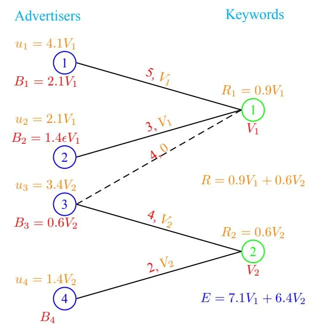
Figure 8: No Shift in Equilibrium due to the new edge (3,1). The values shown along edge (i, j) is(si,j , Vi,j ). uⁱ denote total payoff of advertiser i.

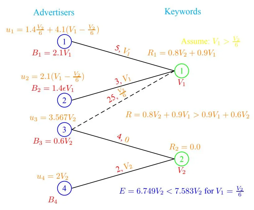
Figure 9: A Shift in Equilibrium due to the new edge (3,1). The values shown along edge (i, j) is (si,j , Vi,j ). uⁱ denote total payoff of advertiser i.

6 Auctioneer Controlled Broad Match(AcBM)

In this section we study the second broad match scenario i.e. AcBM as described in section 4. First, we need a few definitions.

Definition 10 Excess Budget: Let $G = (\mathcal{N}, \mathcal{M}, \mathcal{E})$ be a BMG and $G' = (\mathcal{N}, \mathcal{M}, \mathcal{E}')$ be an extension (broadmatch) of G. For an $i \in \mathcal{N}$ , let $D_i$ denote the budget of i unspent in G and let $s_i = \max_{j \in \mathcal{E}} s_{i,j}$ . We say that i has an excess budget in G iff $s_i \leq D_i$ .

Intuitively, what we mean by an advertiser to have an excess budget is that she has enough amount currently left unspent so that she can participate in at least one query of any of the keywords she is currently bidding on, if given a chance, irrespective of the valuations of her competitors.

Definition 11 Revenue Improving Broad-Match: An extension $G' = (\mathcal{N}, \mathcal{M}, \mathcal{E}')$ of BMG $G = (\mathcal{N}, \mathcal{M}, \mathcal{E})$ is called revenue improving if there exist an allocation of the excess budgets along new edges (i.e. edges in $\mathcal{E}' \setminus \mathcal{E}$ ) so that the sum of total budget spent by all the advertisers is more in G’ than in G, as well as, there is a strongly polynomial time algorithm to find such an allocation of the excess budgets.

Now, for a keyword j, let I(j,l) denote the set of advertisers having sufficient budget to participate in the lth query of this keyword. The following lemma can be obtained in a way similar to the Lemma 1 and again utilizing the partition structure per this lemma, we obtain Observation 13 that as long as the quality of broad-match is good in some sense, the auctioneer can guarantee a better revenue for himself by suitably exploiting the extension.

Lemma 12 Given the budget splitting of all the advertisers for the BMG $G = (\mathfrak{N}, \mathfrak{M}, \mathcal{E})$ (i.e. the current budget splitting ), that is the values $B_{i,j}$ ‘s for all $(i,j) \in \mathcal{E}$ , there exist non-negative integers $\Lambda_j$ , $z_{j,0}, z_{j,1}, z_{j,2}, \ldots, z_{j,\Lambda_j}$ , and sets $I_{j,1}, I_{j,2}, \ldots, I_{j,\Lambda_j}$ , $I_j$ for all $j \in \mathcal{M}$ such that $\Lambda_j = O(N)$ and for all $0 \leq \lambda \leq \Lambda_j - 1$ , $c(i,j,l) = C(i,j,\lambda), I(j,l) = I_{j,\lambda+1} \ \forall z_{j,\lambda} < l \leq z_{j,\lambda+1}$ where $C(i,j,\lambda) := c(i,j,z_{j,\lambda}+1), I_{j,\lambda+1} := I(j,z_{j,\lambda}+1)$ and $I_j = \{i \in \mathcal{N} : (i,j) \in \mathcal{E}, i \text{ has an excess budget in } G\}$ . Moreover, all these $\Lambda, z, C, I$ values can be computed together in time polynomial in N, M and K.

Observation 13 Let $G' = (\mathcal{N}, \mathcal{M}, \mathcal{E}')$ be an extension of BMG $G = (\mathcal{N}, \mathcal{M}, \mathcal{E})$ , $I = \bigcup_{j \in \mathcal{M}} I_j$ , $J_i = \{j \in \mathcal{M} : (i,j) \in \mathcal{E}' \setminus \mathcal{E}\}$ for $i \in I$ , $\Gamma_j = \{i \in \mathcal{N} : (i,j) \in \mathcal{E}'\}$ , and $\Phi = \{j \in \mathcal{M} : I_{j,\Lambda_j} = \phi\}$ . This extension is revenue improving if there is an $i \in I$ having one or more of the following properties/conditions:

• a) $\exists j \in J_i \setminus \Phi$ such that $I_{j,\Lambda_j} = I_j$ and $|\{m \in I_{j,\Lambda_j} : s_{m,j} > s_{i,j}\}| < K$ .
• $\textit{b)} \ \exists j \in J_i \cap \Phi \ \textit{such that} \ | \ \{l \in I \cap \Gamma_j : s_{l,j} = s_{i,j}\} \cup \{l \in \Gamma_j : s_{l,j} < s_{i,j}\} \ | \ > 1.$
• c) $\exists j \in J_i \setminus \Phi$ such that $I_{j,\Lambda_j} \neq I_j$ and $s_{i,j} > \max_{l \in I_{j,\Lambda_j} \setminus I_j} s_{l,j}$ .

Intuitively, the properties a) and c) says that there is an advertiser i with excess budget in G and a keyword j such that i has a good enough valuation for j in G’ so as to obtain a slot, and moreover if i is brought in for the last query, all advertisers already participating in that query have still enough budget to participate in that query. The condition b) says that there is a keyword j with unsold queries in G and we can sell these queries in G’ to at least two advertisers¹³. Thus, these conditions allow the auctioneer to bring additional advertiser(s) for the keyword j to j’s last query or equivalently the very first query in the last partition

^&lt;sup>13Note that just selling to one advertiser does not generate any money in GSP. In practice, however Google/Yahoo! charges a minimum amount i.e. a reserve price for the last slot. Nevertheless, all the results we present remains unchanged by introducing reserve prices for the last slot. In that case, the condition b) will change to $\exists j \in J_i \cap \Phi$ .

((zj,Λj−¹ + 1)th query) so that revenue extracted from this particular query is improved without changing the revenue generated from any other query. Therefore, in terms of the existence of a revenue improving extension we have the above observation. Nevertheless, in general the auctioneer can do much more than the above trivial way. In particular, there might be several i and j’s satisfying the properties in Observation 13 and he could exploit this profitably. Recall that he has a finer control over which query to start with and whatever part of excess budget he can spend along edges in E ′ \ E. So his task is to choose splitting of excess budgets along new edges as well as to decide a starting query number. In general, there could be O(N) advertisers with excess budgets and there could be O(MN) new edges, finding the best splitting is a variant of Integer Knapsack problem again and thus computationally hard. Nevertheless, it is clearly possible to design strongly polynomial time sub-optimal algorithm that does significantly better than the trivial improvement possible by increasing competition for the last query. The problem with participating starting a query in other partitions is that it may change the partition structure in a way that is not revenue improving, but since there are only O(N) such partitions for each keyword, we could check for each partition whether starting with its first query is revenue improving or not. Indeed, it is easy to think of a strongly polynomial time algorithm that finds excess budget splittings which improves revenue, one that moves from partition to partition, taking starting query as the first query in that partition and then doing a binary search for appropriate budget (as high as possible) to be allocated and tracks which one of these possibilities lead to the highest revenue. Note that since we are doing a binary search on budget (and equivalently on the number of queries to participate in), we are still in strongly polynomial time regime. Finally, it should be interesting to search for efficient algorithms generating better revenue and in particular a FPTAS, possibly by efficiently searching for which query to start with along with efficiently searching for how many queries to participate for.

Now, given that auctioneer’s goal is primarily to improve revenue, we should also analyze what happens to the efficiency (i.e. social welfare), if the auctioneer implements such revenue improving broad-match. First, it is clear that if auctioneer’s goal were to improve social welfare instead of revenue, he could certainly do so in a way similar to the one discussed above for revenue improvement. Moreover, revenue and social welfare could infact be improved together if one of the conditions in Observation 13 holds and the proof is same as that for Observation 13 by bringing in appropriate advertiser(s) in the last query of an appropriate keyword. However, if auctioneer deviates from this trivial way of improving revenue, which infact he will do if his goal is to maximize revenue, there can often be a tradeoff with social welfare. For an explicit example of this tradeoff please refer to Figure 10. Furthermore, even when the conditions in Observation 13 are NOT satisfied, there might still be a possibility of revenue improvement (ref. Figure 1).

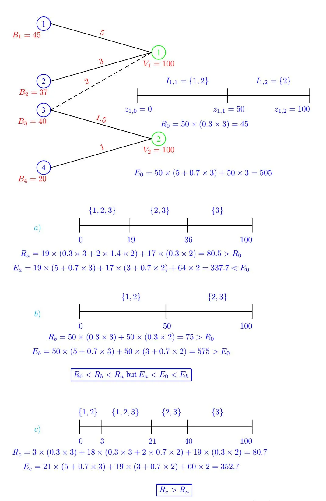
Figure 10: Tradeoff in revenue and social welfare, the base BMG does not include edge (3,1), its extension does. The revenue and efficiency value is just for keyword 1, as these values do not change for keyword 2 even in the extension. In a) and b) advertiser 3 is brought in for keyword 1 starting with first query in partition 1 and 2 respectively. Note that the choice of partition with better revenue is the one where efficiency decreases. c) shows that just starting with the first query of a partition may not lead to optimal revenue, for example if 3 is started with 4th query then the revenue improvement is even better than a) or b).

7 Future Directions

We have initiated a study of broad-match, an interesting aspect of sponsored search advertising, and as common to papers that initiate a new direction of study, this paper leaves out several important open problems that deserve theoretical investigation and analysis. We discuss some of these interesting problems in the following.

Budget Splitting Games(BSG): Abstracting the settings in Broad-Match Game can provide us with a rich class of mutli-player games having compact representations. It should be interesting to study these games and to consider the budget splitting/allocation scenarios beyond the currently prevailing models for sponsored search advertising, as well as, other interesting applications. Herebelow we provide an abstraction.

An instance of BSG is given by (N,M, E, B, V, O). N is the set of players, M is set of distinct type of indivisible items and (N,M, E) is a bi-partite graph between the players and items wherein an (i, j) ∈ E iff the player i ∈ N is interested in buying the item j ∈ M (i.e. i have a positive valuation for j). B = {Bi}i∈^N is the budget vector, Bⁱ being the total budget of player i. V = {Vj}j∈^M is the volume vector, V^j being the total number of units of the item j for sale. Let |N| = N and |M| = M. O is an oracle that takes as input (i, j) ∈ E and a set of budget values {Bn,j}n∈N−{i} and output the set of values Λ^j = O(N), zj,⁰ = 0, zj,1, zj,2, … , zj,Λ^j = V^j , and C(i, j, λ), U(i, j, λ) for all 0 ≤ λ ≤ Λ^j − 1, to be interpreted as follows: given that for all n ∈ N − {i}, the player n spends/allocates an amount Bn,j on the item j, C(i, j, λ) and U(i, j, λ) respectively are the cost and the utility for each unit of the item if the player i decides to buy zj,λ < Vi,j ≤ zj,λ+1 units of the item j. Each player has access to the oracle O. The strategy of a player i is to split her budget across various items that is to choose the values {Bi,j}j∈M:(i,j)∈^E such that P ^j∈M:(i,j)∈EBi,j ≤ Bⁱ and correspondignly the number of units of the various items {Vi,j}j∈M:(i,j)∈^E with Vi,j ≤ V^j . The payoff of a player is the total utility it derives across all the items from their units she bought as per her chosen strategy.

Note that this abstraction nicely captures the Broad-Match Game studied in the present paper wherein an item is a keyword and a query of a keyword corresponds to a unit. The oracle O corresponds to the Lemma 1. Further, by varying the properties satisfied by the values C(i, j, λ), U(i, j, λ)‘s we may obtain other interesting scenarios.

Complexity of Auctioneer’s Dilemma: The Theorem 9 leaves the auctioneer in a dilemma about whether he should broad-match or not. If he could somehow predict which choice of broad match lead to a revenue improvement for him and which not, he could potentially choose the ones leading to a revenue improvement. This brings forth one of the big questions left open in this paper, that is of efficiently computing a BME / ǫ*-NE*, if one exists, given a choice of broad match, as well as, to efficiently decide whether a given broad match is revenue improving or not in the AdBM scenario.

Existence of pure NE/ǫ-NE/BME in Broad-Match Game: Despite some effort we have not been able to show that a Broad-Match Game always admits pure NE or even ǫ-NE or BME. On the other hand we have also not been able to construct examples where they do not exist. The problem arises from the fact that the payoff funtions are discontinuous and not even quasi-concave. Therefore, the existing techniques or their simple extensions do not seem to work. This calls for developing new techniques for proving the existence of pure Nash equilibria and the complexity of deciding the existence in general, and for the Broad-Match Game and BSGs in particular.

Quantifying the Effect of Broad-Match: As per various observations including Theorem 9 obtained in the Section 5.4 we know that the the revenue of the autioneer and the social welfare could very well degrade by incorporating broad-match and it would be interesting to characterize the extent of such degradation.

Total Click-Through-Rates as Payoff: It would be interesting to analyze the effect of broad-match in a scenario where the advertisers are interested in maximizing their total Click-Through-Rate across various keywords rather than their total utilities. Note that the budget splitting game arising in this sceneario indeed fits in our abtract model of BSG discussed earlier in this section. With the intuition developed from this paper, we believe that similar conclusions hold true even in the case of total Click-Through-Rates as payoffs.

BME vs ǫ**-NE:** As we argued in the paper, both the BME and ǫ*-NE* are reasonable solution concepts for the Broad-Match Game. Further, we constructed examples where the both solution concepts coincide. Nevertheless, it would be nice to study these two concept comparatively at a finer level. For example, BME may not provide good approximation guarantee to the advertisers but it demands less shophistication level from them than that required for good approximation guarantee.

Network Level Competition via Broad-Match Game: The framework provided in the present paper is easily applicable to the scenario where advertisers are trying to optimally split budgets across various keywords coming from several competing search engines. How does the revenue of one search engine gets effected by the fact that another competeting search engine offers broad-match? For example consider the BMG in the Figure 9, without the dashed edge (3, 1), and suppose that the keyword 1 is coming from the search engine 1 and the keyword 2 is coming from the serach engine 2. Now if the search engine 1 does broad-match and introduces the new edge (3, 1) then we can see that the revenue of the search engine 1 increases whereas that of search engine 2 decreases. It should be interesting to further explore this direction.

Formalizing a Notion of “Good” Broad-Match: In the analysis we have presented, we have not considered costs incurred by the auctioneer in the short run due to uncertainty about the extended part of the BMG, although we can expect that as long as the quality of broad match being performed is good, such costs should be minimal. Nevertheless, formalizing a notion of good broad match should be interesting. Features such as the improvement in the relevance scores and conversion rates should be an essential ingredient of a good broad match. Further, the conditions noted in the Observation 13 also provides some sense of what should be the features of a good broad-match from the viewpoint of the auctioneer.

Acknowledgements: We thank Gunes Ercal, Himawan Gunadhi, Adam Meyerson and Behnam Rezaei for discussions and anonymous reviewers of an earlier version for valuable comments and suggestions. SKS thanks Zo¨e Abrams, Arpita Ghosh, Gagan Goel, Jason Hartline, Aranyak Mehta, Hamid Nazerzadeh, and Zoya Svitkina for useful discussions during WINE 2007.

References

• [1] G. Aggarwal, A. Goel, R. Motwani, Truthful Auctions for Pricing Search Keywords, EC 2006.

• [2] C. Borgs, J. Chayes, N. Immorlica, K. Jain, O. Etesami, and M. Mahdian, Dynamics of bid optimization in online advertisement auctions, WWW 2007.

• [3] M. Cary, A. Das, B. Edelman, I. Giotis, K. Heimerl, A. R. Karlin, C. Mathieu, and M. Schwarz, Greedy bidding strategies for keyword auctions, EC 2007.

• [4] B. Edelman and M. Ostrovsky, Strategic bidder behavior in sponsored search auctions, Decis. Support Syst., 43(1):192-198, 2007.

• [5] B. Edelman, M. Ostrovsky, M. Schwarz, Internet Advertising and the Generalized Second Price Auction: Selling Billions of Dollars Worth of Keywords, American Economic Review, 97(1):242-259, 2007.

• [6] J. Feldman, S. Muthukrishnan, M. Pal, and C. Stein, Budget optimization in search-based advertising auctions, EC 2007.

• [7] R. Gonen and E. Palkov, An Incentive-Compatible Multi-Armed Bandit Mechanism, PODC 2007.

• [8] O. H. Ibarra and C. E. Kim, Fast Approximation Algorithms for the Knapsack and Sum of Subset Problems, JACM , Vol. 22, pp:463 - 468 , 1975.

• [9] S. Lahaie, An Analysis of Alternative Slot Auction Designs for Sponsored Search, EC 2006.

• [10] E. L. Lawler, Fast Approximation Algorithms for Knapsack Problems Mathematics of Operations Research, Vol. 4, pp: 339-356, 1979.

• [11] S. Lahaie, and D. Pennock, Revenue Analysis of a Family of Ranking Rules for Keyword Auctions, EC 2007.

• [12] A. Mehta, A. Saberi, U. Vazirani, and V. Vazirani, AdWords and generalized on-line matching, FOCS 2005.

• [13] S. Muthukrishnan, M. P´al, and Z. Svitkina, Stochastic Models for Budget Optimization in Search-Based Advertising, WINE 2007.

• [14] C. H. Papadimitriou, The Complexity of Finding Nash Equilibria, Chapter 2, Algorithmic Game Theory, Cambridge University Press, 2007.

• [15] C. H. Papadimitriou, and T. Roughgarden, Computing Equilibria in Multi-Player Games, SODA 2005.

• [16] C. H. Papadimitriou, and K. Steiglitz, Combinatorial Optimization: Algorithms and Complexity, Dover Publications 1998.

• [17] T. Roughgarden, Selfish Routing and the Price of Anarchy, MIT Press, 2005.

• [18] P. Rusmevichientong, and D. P. Williamson, An adaptive algorithm for selecting profitable keywords for search-based advertising services, EC 2006.

• [19] S. K. Singh, V. P. Roychowdhury, M. Bradonji´c, and B. A. Rezaei, Exploration via design and the cost of uncertainty in keyword auctions, Submitted.

• [20] S. K. Singh, V. P. Roychowdhury, H. Gunadhi, and B. A. Rezaei, Capacity Constraints and the Inevitability of Mediators in Adword Auctions, WINE 2007.

• [21] S. K. Singh, V. P. Roychowdhury, H. Gunadhi, and B. A. Rezaei, Diversification in the Internet Economy:The Role of For-Profit Mediators, Submitted.

• [22] H. Varian, Position Auctions, International Journal of Industrial Organization, 25(6):1163-1178, 2007.

• [23] V. V. Vazirani, Approximation Algorithms, Springer 2001.

• [24] J. Wortman, Y. Vorobeychik, L. Li, and J. Langford, Maintaining equilibria during exploration in sponsored search auctions, WINE 2007.